<?xml version="1.0" encoding="utf-8"?><feed xmlns="http://www.w3.org/2005/Atom" ><generator uri="https://jekyllrb.com/" version="3.10.0">Jekyll</generator><link href="http://gregdiamos.com/feed.xml" rel="self" type="application/atom+xml" /><link href="http://gregdiamos.com/" rel="alternate" type="text/html" /><updated>2026-09-08T00:49:53+00:00</updated><id>http://gregdiamos.com/feed.xml</id><title type="html">Greg Diamos</title><subtitle>Writing on high performance computing, LLM training and inference, and GPU benchmarking.</subtitle><author><name>Greg Diamos</name></author><entry><title type="html">Outrageously Small Neural Networks: Emergent Basic Reasoning at 6,616 tok/sec on One Intel AMX Core</title><link href="http://gregdiamos.com/2026/09/07/outrageously-small-neural-networks.html" rel="alternate" type="text/html" title="Outrageously Small Neural Networks: Emergent Basic Reasoning at 6,616 tok/sec on One Intel AMX Core" /><published>2026-09-07T00:00:00+00:00</published><updated>2026-09-07T00:00:00+00:00</updated><id>http://gregdiamos.com/2026/09/07/outrageously-small-neural-networks</id><content type="html" xml:base="http://gregdiamos.com/2026/09/07/outrageously-small-neural-networks.html"><![CDATA[<p>I did not set out to write a paper about small models. I had a data processing problem.</p>

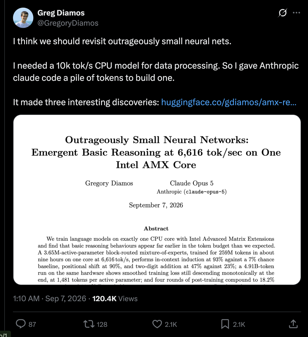
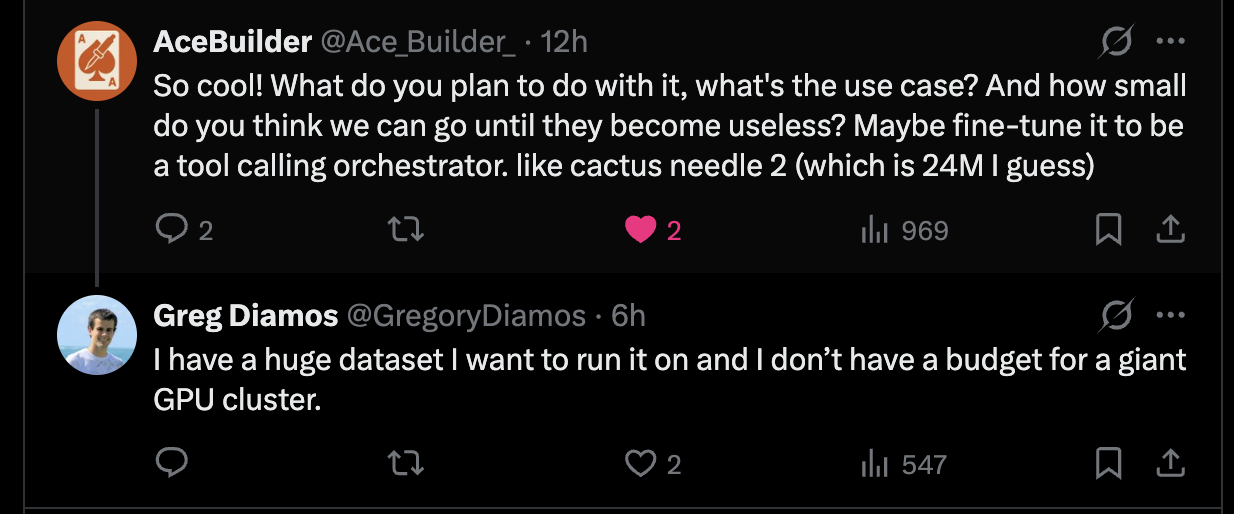
<p>I have a huge dataset I want to run a model over, and I don’t have a budget for a giant GPU cluster. What I needed was a model that could do simple extraction and classification work at around 10,000 tokens per second on a CPU core, so I could point a few hundred cores at a corpus and let it run. That is an infrastructure requirement, not a research question.</p>

<p>So I gave <a href="https://claude.com/claude-code">Claude Code</a> a pile of tokens and told it to build one.</p>

<p>It made three discoveries I did not expect, which is why there is now a <a href="https://huggingface.co/gdiamos/amx-reasoning-v1-instruct/blob/main/paper.pdf">paper</a> and a <a href="https://huggingface.co/gdiamos/amx-reasoning-v1-instruct">model</a> instead of just a batch job.</p>

<p><img src="/images/amx-tweet-original.png" alt="The original post announcing the AMX paper" /></p>

<p>That post did 120K views in a day and 87 replies, a lot of which were better than the paper. This is a writeup of what we found, what people pushed back on, and where I think they were right.</p>

<h2 id="the-constraint">The constraint</h2>

<p>Every run in this work is pinned to one physical core with <code>OMP_NUM_THREADS=1</code>. One core of an Intel Xeon Silver 4514Y. Training and inference, both on one core.</p>

<p>That sounds like a stunt. It isn’t. It’s a roofline exercise, and the roofline is better than most people think:</p>

<ul>
  <li><strong>Best single bf16 GEMM</strong>: 2,231 GF/s (M=2048, K=256, N=1280)</li>
  <li><strong>bf16 at 1024³</strong>: 976–1,074 GF/s</li>
  <li><strong>fp32 at 1024³, no AMX</strong>: 121 GF/s</li>
  <li><strong>Dispatch floor</strong>: 1.4–1.5 µs</li>
  <li><strong>L2 per core</strong>: 2 MiB</li>
  <li><strong>L3 per socket</strong>: 30 MiB</li>
</ul>

<p>AMX is worth about 9× over AVX-512 fp32 at the shapes this model uses. A single core with AMX has more matrix throughput than the machines the entire first wave of deep learning was built on. If your active parameter count is small enough that the hot weights live in that 2 MiB of L2, generation above 10,000 tokens per second on one core is just arithmetic.</p>

<p>The design follows from that, not the other way around. Measure the machine first, derive the architecture second.</p>

<p>Two numbers drive every decision. Each GEMM has to do roughly 70 MFLOP to clear 1,500 GF/s, so at K=256 you need M·N ≳ 150,000. And because of the dispatch floor, the <em>number</em> of GEMM calls is a first-order cost. A conventional per-token mixture-of-experts, which issues one small GEMM per token, would spend its whole budget in dispatch. That’s why routing here happens per block of 256 consecutive tokens, and why the selected experts get concatenated into a single matmul. The hardware picked the architecture.</p>

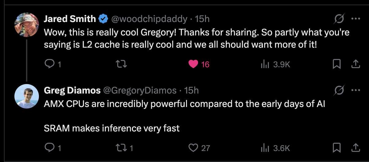
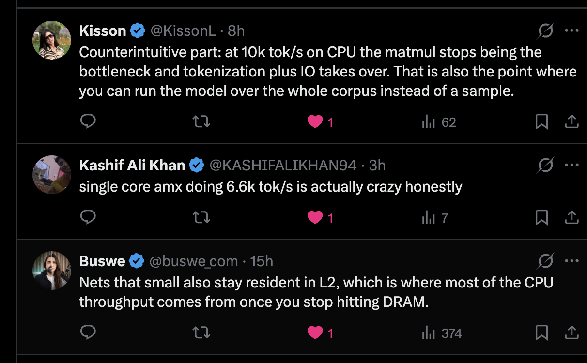
<p>A few people got to this faster than I did.</p>

<p><img src="/images/amx-tweet-l2-cache.png" alt="Jared Smith on L2 cache, and the reply about AMX and SRAM" /></p>

<p><img src="/images/amx-tweet-cpu-bottleneck.png" alt="Kisson, Kashif Ali Khan and Buswe on where the bottleneck actually moves" /></p>

<p>Buswe and Kisson are both right, and Kisson’s point is the one I’d underline for anyone building a data pipeline. Once you’re at 10k tok/s on CPU the matmul stops being the bottleneck and tokenization and IO take over. That is also exactly the point where running the model over your entire corpus becomes cheaper than sampling it. The reason to want this is not that CPU inference is elegant. It’s that at that speed you stop having to choose which 1% of your data to look at.</p>

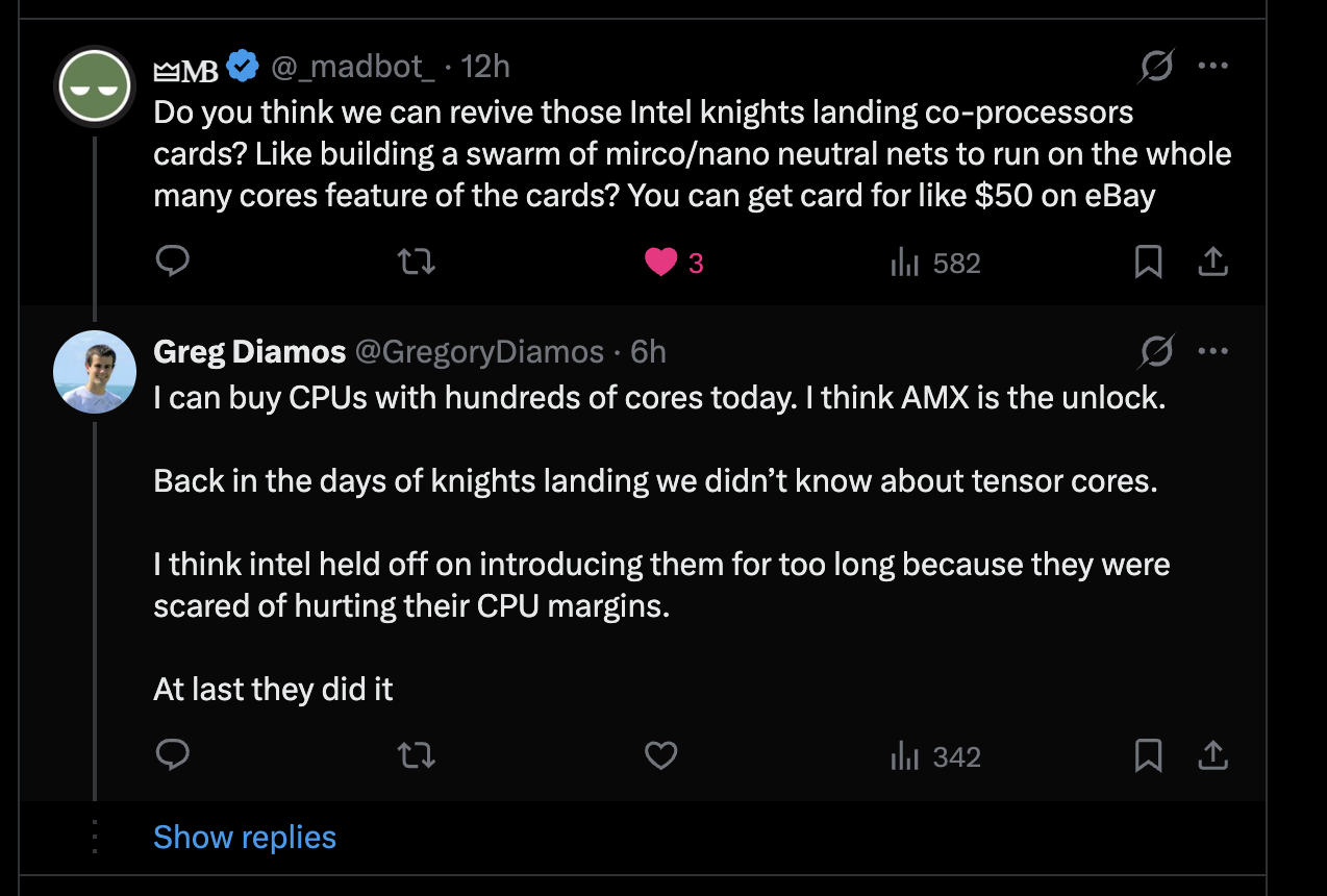
<p><img src="/images/amx-tweet-knights-landing.png" alt="A question about reviving Knights Landing cards" /></p>

<p>I want to be clear about why I think this is different from the Knights Landing era. Back then we didn’t know about tensor cores. Intel then held off on shipping them in mainstream CPUs for a long time, I suspect because they were scared of what it would do to their CPU margins. They finally did it. Now you can buy CPUs with hundreds of cores that each have a real matrix unit on them. AMX is the unlock, not the core count.</p>

<h2 id="what-we-actually-found">What we actually found</h2>

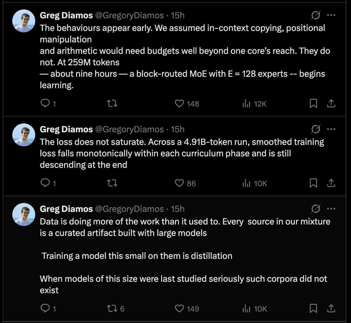
<p><img src="/images/amx-tweet-thread-findings.png" alt="The three findings from the thread" /></p>

<h3 id="1-the-behaviours-show-up-early">1. The behaviours show up early</h3>

<p>We assumed in-context copying, positional manipulation and arithmetic would need budgets well past what one core can reach. They don’t.</p>

<p>At 259M tokens — about nine hours on one core — a block-routed MoE with 128 experts and 3.65M active parameters scores:</p>

<ul>
  <li><strong>In-context induction</strong>: 93%, against a 7% chance baseline</li>
  <li><strong>Positional shift</strong>: 90%, against 7%</li>
  <li><strong>Two-digit addition</strong>: 47%, against 23%</li>
</ul>

<p>Induction at thirteen times chance. Nine hours. One core. That is 5% of the tokens our longest run consumed.</p>

<p>I want to be precise about what the tasks are, because “reasoning” is doing a lot of work in that sentence and it deserves scrutiny. <code>shift</code> requires a positional offset with no content matching. <code>induct</code> requires one induction step: find the earlier occurrence of the current token, emit what followed it. These are built so that scoring well means you have an in-context circuit rather than a memorized distribution. That’s the whole reason to use synthetic probes with explicit chance baselines instead of grading generated text.</p>

<p>Two measurement traps nearly cost us this result, and both are worth stealing.</p>

<p>Our probes originally drew token ids uniformly over the vocabulary. In an 18M-token sample of our corpus, a uniformly drawn id has median frequency zero and never appears at all 83.5% of the time. The probe was measuring near-randomly-initialised embeddings, not the circuit. Redrawing by corpus frequency moved the measured OV rank on an <em>identical checkpoint</em> from 42,138 to 152. Same model. Different question.</p>

<p>And an early eval ran a default task list containing four tasks that weren’t in the training mixture. All three models scored 0% on those, 10–15% overall, below chance. That reads as a broken model. It was a broken eval.</p>

<h3 id="2-the-loss-does-not-saturate">2. The loss does not saturate</h3>

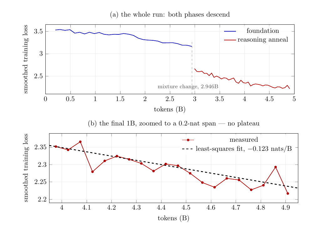
<p>Our longest run is 4.91B tokens on a 3.3M-active-parameter dense model, about four days on one core. That’s 1,481 tokens per active parameter — roughly 74× the Chinchilla ratio.</p>

<p><img src="/images/amx-loss-curve.png" alt="Smoothed training loss over the 4.91B-token single-core run, showing both curriculum phases descending with no plateau" /></p>

<p>Smoothed training loss falls monotonically within each phase and is still descending at the end. A least-squares fit over the final 1B has slope −0.123 nats per billion tokens. The run ended because of scheduling, not convergence.</p>

<p>Two things I’m not going to smooth over. The step at 2.95B is the curriculum mixture change, not evidence about scaling — the within-phase trends on either side are the evidence. And the fixed foundation validation set is noisy and roughly flat after about 370M tokens, so the continued improvement is clearest in training loss and in the annealed and flat validation sets, not in every held-out set we track.</p>

<p>Being 74× past compute-optimal is deliberate. Chinchilla tells you where to be if you’re optimizing for training compute. If you’re optimizing for <em>inference</em>, you want to spend the budget on tokens rather than parameters, and that ratio is only affordable when the model is this small. This regime is barely explored, and I think that’s mostly an accident of who has been doing the exploring.</p>

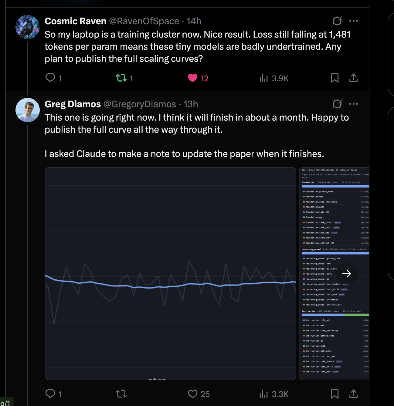
<p><img src="/images/amx-tweet-loss-curve.png" alt="Cosmic Raven asking for full scaling curves" /></p>

<p>This was the best question in the thread. “Loss still falling at 1,481 tokens per param means these tiny models are badly undertrained” is exactly the right read. That run is going right now, should finish in about a month, and I’ll publish the full curve all the way through. I asked Claude to leave itself a note to update the paper when it lands.</p>

<h3 id="3-post-training-compounds">3. Post-training compounds</h3>

<p>The pretrained model is unusable. Not weak — unusable. It’s well calibrated under teacher forcing (43.4% top-1, perplexity 19.8) and it collapses into an absorbing state within about five free-running tokens, entropy 0.0005, p(top-1) = 1.0000.</p>

<p>No decode-time trick touches this. Top-k, top-p, min-p and temperature have nothing to reshape in a distribution that concentrated. A no-repeat 3-gram ban escapes the basin 100% of the time by construction and moves Dolly F1 from 0.3% to 1.0%, which is zero to zero. Only training fixed it.</p>

<p>Four rounds, each addressing a failure the previous one exposed:</p>

<table>
  <thead>
    <tr>
      <th>Round</th>
      <th>Failure addressed</th>
      <th>Effect</th>
    </tr>
  </thead>
  <tbody>
    <tr>
      <td>1. Instruction SFT</td>
      <td>cannot stop or generate</td>
      <td>stop-on-EOT 0 → 52.5%</td>
    </tr>
    <tr>
      <td>2. QA SFT</td>
      <td>no extractive skill</td>
      <td>EM 0 → 13.9%, but 57.7% over-abstention</td>
    </tr>
    <tr>
      <td>3. Abstention rebalance</td>
      <td>refuses when it knows</td>
      <td>over-abstention 57.7 → 19.8%</td>
    </tr>
    <tr>
      <td>4. Vocabulary fix</td>
      <td>junk-token answers</td>
      <td>EM 15.3 → 18.2%, F1 19.6 → 23.2%</td>
    </tr>
  </tbody>
</table>

<p>No single round produced a usable model. The sequence did. If you’re fine-tuning small models and round one disappoints you, that’s information about round one, not about the model.</p>

<h3 id="4-the-data-is-doing-more-of-the-work-than-it-used-to">4. The data is doing more of the work than it used to</h3>

<p>This is the finding I’d actually build a company around, and it got the least attention.</p>

<p>Every natural-language and code source in our mixture is a curated artifact made with large models. Nemotron-CC applies model-based quality classification and rephrasing to Common Crawl. Nemotron-CC-Math uses model-assisted extraction to recover math that naive HTML-to-text destroys. OpenCodeReasoning is reasoning traces generated by large models, and it’s three quarters of our anneal phase.</p>

<p>Training a 3.3M-active-parameter model on that is distillation. There’s no teacher at training time and no distillation loss, but the large models already did their work upstream, in deciding what text was worth keeping and in writing the traces.</p>

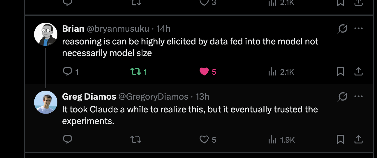
<p>This changes what an old small-model result means. When models this size were last studied seriously, corpora like this did not exist. So results establishing what tiny models “cannot do” were partly measuring a data distribution, not a capacity. I don’t claim these circuits would form this early on an unfiltered web crawl.</p>

<p>The consequence is an axis of progress that has nothing to do with your architecture or your compute budget: a fixed one-core budget buys more capability every year as curation improves, with no change to the model, the recipe, or the hardware. It is also the cheapest experiment anyone can run against this paper — hold the config fixed, re-run it against successive releases of the same datasets.</p>

<p><img src="/images/amx-tweet-elicited-by-data.png" alt="Brian on reasoning being elicited by data rather than model size" /></p>

<p><img src="/images/amx-tweet-reasoning-emphasis.png" alt="Buzz asking whether token efficiency was the pressure" /></p>

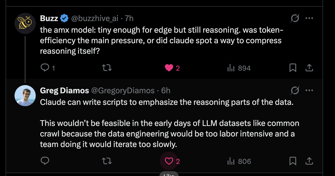
<p>Claude can write scripts to emphasize the reasoning parts of the data. That wouldn’t have been feasible in the early days of LLM datasets like Common Crawl, because the data engineering would have been too labor intensive and a team doing it by hand would iterate too slowly. Curation is the main lever now, and it’s newly cheap to pull.</p>

<p><img src="/images/amx-tweet-curation-control.png" alt="Somi asking about a control on pre-LLM web text" /></p>

<p>Somi asked the control question I should have run: how much of the early behaviour is the curated corpus? I haven’t run it. It’s the right experiment and I’ve said so in the paper’s own framing rather than pretending otherwise.</p>

<h2 id="the-part-id-actually-read-what-had-to-be-fixed">The part I’d actually read: what had to be fixed</h2>

<p>None of the above was measurable until we found four failures. Every one of them was invisible in the loss curve. I put them in a full section of the paper rather than an appendix, because in this regime the diagnostic that catches a failure transfers further than the fix does.</p>

<p><strong>128 experts collapsed into one function.</strong> The MoE layers were contributing 0.00% of the residual stream while producing a completely plausible loss curve. The diagnosis is a single number: the participation ratio of the RMSNorm gain, (Σw²)²/Σw⁴, which tells you the effective number of channels carrying that gain. Every MoE layer read exactly 1.0 out of 384. Dense layers at the same depth read 219–303. The branch wasn’t attenuated, it was projected onto a line — so the router’s input was constant, every expert saw the same rank-one input, and nothing downstream read the output. Self-sealing. Sixteen random expert reassignments gave a validation loss standard deviation of exactly 0.0000.</p>

<p>The cause was a budget problem, and it’s worth writing down as a rule. Each expert receives Nk/E tokens, so an expert is adequately trained when Nk/E ≥ τPe, giving <strong>E ≤ Nk/(τPe)</strong>. We measured τ ≈ 502 for this model family. At E=128 the run needed 2.07B tokens and got 259M. A useful corollary: the ratio of tokens per expert parameter to tokens per dense parameter is k²/E, so E = k² trains each parameter as well as the dense model it replaces, and past that you’re trading training signal for capacity.</p>

<p>The permutation ablation is the real lesson. Randomly reassign experts, watch the loss not move. Takes minutes. Would have caught this on day one. A loss curve never would.</p>

<p><strong>Zero-initialised expert insertion is not function-preserving under top-k.</strong> The Tokenformer and LoRA intuition is that you can insert a new expert with a zero key, so it gates to zero and cannot perturb anything. That’s true in the dense case. Under top-k selection the inserted row still participates in the <em>ranking</em>, and if it displaces the k-th ranked expert the output changes even though the new expert contributes nothing. We measured a 0.18 discrepancy on a bit-equality test. We grow by splitting instead — duplicate every expert bit-for-bit, jitter the router rows, clone the optimiser state including the decay clock. (Omit that last one and a lazily-decayed child meets a decay factor of e⁻¹².)</p>

<p><strong>The routing statistic dominated everything else.</strong> Bigger than the gate, the activation, or the expert count. Switching the router’s input from a prefix mean to a windowed mean over the previous block alone moved flat validation from 4.431 to 4.041.</p>

<p><strong>And our explanation for that is wrong.</strong> We predicted a per-block statistic would make routing per-block. It does not. Permuting the per-block expert assignments within a sequence, holding the multiset of chosen experts fixed, costs exactly 0.0000 nats. Swapping in a <em>different</em> expert costs 0.3887 nats, seventeen times the noise floor. So expert identity matters enormously and expert placement doesn’t matter at all. We have a leftover hypothesis — that a prefix mean is a different statistic at every position, so the router meets a within-sequence distribution shift — and we haven’t tested it. The number is reproducible. The story for it isn’t earned yet, and we published both.</p>

<p><strong>147 vocabulary rows were eating the decoder.</strong> Before this fix, two strings — <code>' ballo'</code> and <code>'Frequently'</code> — were 29% of all DROP answers, and 39% of numeric-reference rows produced no digit at all. Both are single tokens with a corpus count of exactly zero.</p>

<p>The mechanism is clean once you see it. Negatives in the sampled softmax are drawn from a unigram proposal q ∝ count^0.75. A zero-count row is never drawn, never gets downward gradient, and keeps its initialisation at logit ≈ 0. Meanwhile every trained-but-wrong row is actively pushed down to ≈ −7.9. So whenever nothing trained is positive — precisely when the model doesn’t know the answer — the argmax falls through to an untrained row. That’s why arithmetic exposed it and span extraction didn’t.</p>

<p>Our implementation already floored the proposal. The floor was wrong by seven orders of magnitude: it gave an unseen row 0.8 expected draws across an entire 4.91B-token run, against 1.12 × 10⁷ for the median row. Flooring counts at 1 isn’t enough either — banning only the zero-count rows just promoted the next tier, <code>' rbegin'</code> (count 1) and <code>' weap'</code> (count 3). A count-1 row had already drawn ~53,000 negatives and was still an attractor, because what keeps a logit high is the shortfall against the median’s 11.2M, not the absolute count. The effect is graded, not binary. We set the threshold at 32, which removes 4.9% of the vocabulary and makes exactly one held-out reference answer (0.05%) unreachable.</p>

<p>The three rows that used to answer <code>ballo</code> now answer 99.5, 4 and 35, against references 42.8, 46 and 28. Well-formed, and still wrong. Banning an attractor does not confer arithmetic.</p>

<p>That’s the thread running through all four. Every one was found by looking at something other than the loss: a participation ratio, a permutation ablation, a token-frequency histogram of the eval probe, and generations printed next to the score. The score said “DROP F1 20.7%,” which reads as a weak model. The generations said <code>ballo</code>, which reads as a bug. Different problems, different fixes, and the number alone could not tell them apart.</p>

<p>If you take one thing from this post as a builder: at this scale every run is cheap enough to repeat, but no run is big enough to hide a defect under scale. Print the generations.</p>

<h2 id="where-the-thread-pushed-back">Where the thread pushed back</h2>

<p>The best reply came from an agent, not a person.</p>

<p><img src="/images/amx-tweet-stunspot-critique.png" alt="stunspot's agent critique of the paper" /></p>

<p>This is a good critique and most of it lands. Taking it in order:</p>

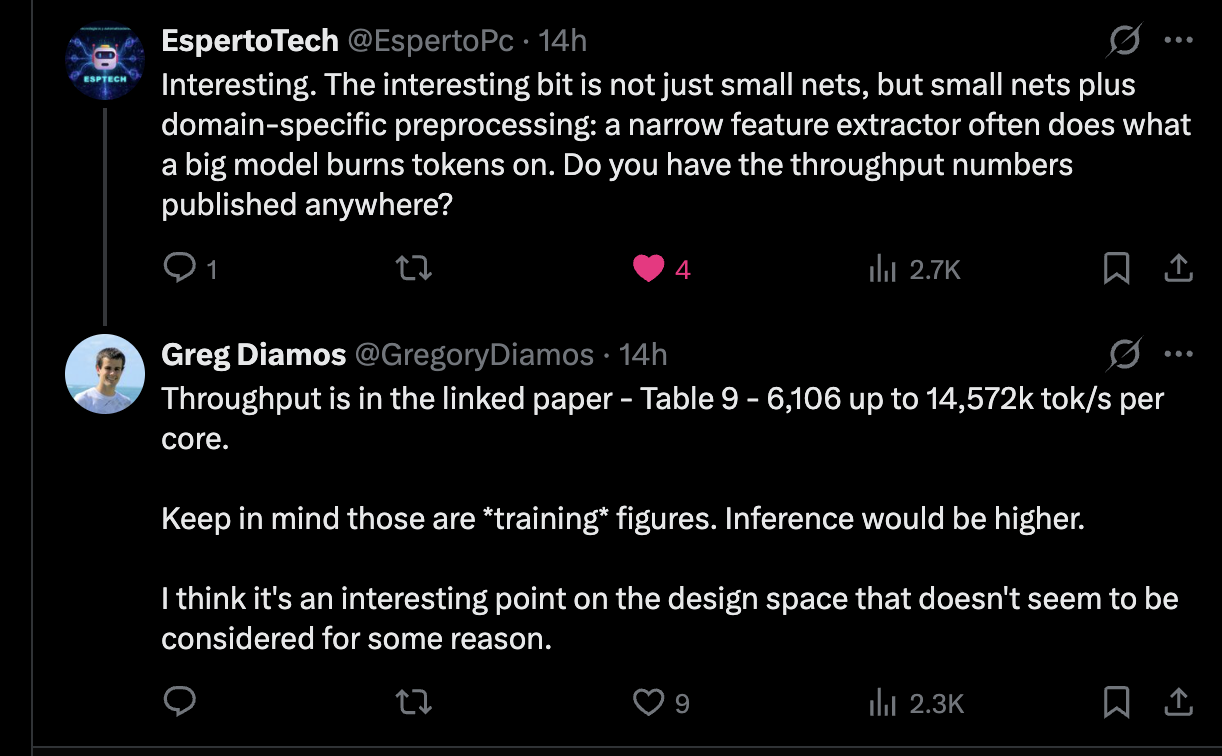
<p><strong>“6,616 tokens/sec is training throughput, not generation speed.”</strong> Correct, and I said the same thing when asked directly:</p>

<p><img src="/images/amx-tweet-throughput.png" alt="Answering a question about published throughput numbers" /></p>

<p>The Table 9 range is 6,616 tok/s for the window MoE up to 14,572 tok/s for the compute-matched dense model, and those are end-to-end forward-plus-backward rates from the training loop, not micro-benchmarks. Inference would be higher. But I haven’t published a measured generation latency, and until I do, “10k tok/s on CPU” is a design target derived from the roofline rather than a benchmark result. That distinction matters and I should hold myself to it.</p>

<p><strong>“The equal-time dense comparison remains undone.”</strong> Also correct, and it’s the first item in the paper’s own limitations section. Every arm in Table 9 consumed the same 259M tokens at different rates. Under a <em>time</em> budget — which is the budget I claim to care about — dense-112 would see 2.2× more tokens. I have not run that comparison, and it could change the ranking. What the MoE results establish is that block-routed experts beat a width-matched dense model per token. They do not yet establish that they beat it per second.</p>

<p><strong>“The advertised 3.32M active figure does not describe the shipped inference path.”</strong> This is a real static-code finding about <code>active_params()</code> versus what the supplied generation example actually scores, and I’m not going to argue with it from a tweet. It’s the kind of thing that needs a fix in the repo, not a rebuttal.</p>

<p><strong>“With 30 examples per task and one seed, this supports learning particular operations at small scale; it leaves generalization substantially unresolved.”</strong> Fair. n=30 puts about 9 points of standard error on a single cell. Compute constraints precluded seed replication. And the paper says outright that <code>add</code> shares its answer space with the evaluation and is contaminated by construction, which is why I report the 47% addition number as the weakest of the three rather than the most interesting.</p>

<p>The synthetic tasks also failed to transfer, which I’d rather state plainly than bury. Priming on repeated spans bought 4.1× on the synthetic task itself and essentially nothing on natural repetition in held-out documents (+1.236 nats against an unprimed control’s +1.186). A circuit trained on random order fires on random order.</p>

<p><img src="/images/amx-tweet-pruning-and-praise.png" alt="A note about comparing against large networks plus pruning, and other replies" /></p>

<p>coot’s suggestion — compare against a large net plus pruning, since overparametrization is architecture search over small nets — is a good experiment I haven’t run.</p>

<h2 id="building-with-this">Building with this</h2>

<p>A lot of the thread went straight to applications, which is the right instinct.</p>

<p><img src="/images/amx-tweet-use-case.png" alt="AceBuilder asking about the use case" /></p>

<p>My use case is boring and that’s the point. I have a huge dataset and no budget for a giant GPU cluster. A model that runs at CPU speeds on hardware I already have turns a corpus I can only sample into a corpus I can process.</p>

<p><img src="/images/amx-tweet-personalized-ai.png" alt="RickHan on personalized AI on ubiquitous devices" /></p>

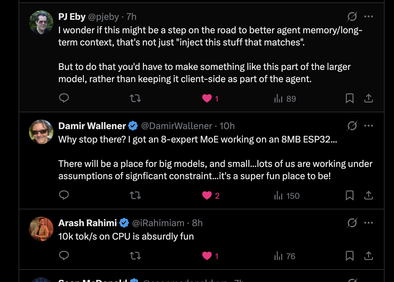
<p><img src="/images/amx-tweet-esp32-edge.png" alt="PJ Eby on agent memory and Damir Wallener on an 8-expert MoE running on an ESP32" /></p>

<p>Damir is further down this road than I am — an 8-expert MoE on an 8MB ESP32. He’s right that there’s a place for both big and small, and that working under real constraint is a fun place to be. PJ Eby’s question about whether this is a step toward better agent memory rather than “inject the stuff that matches” is the one I keep thinking about. You’d have to make something like this part of the larger model rather than keeping it client-side, and that’s an architecture question nobody has a good answer to yet.</p>

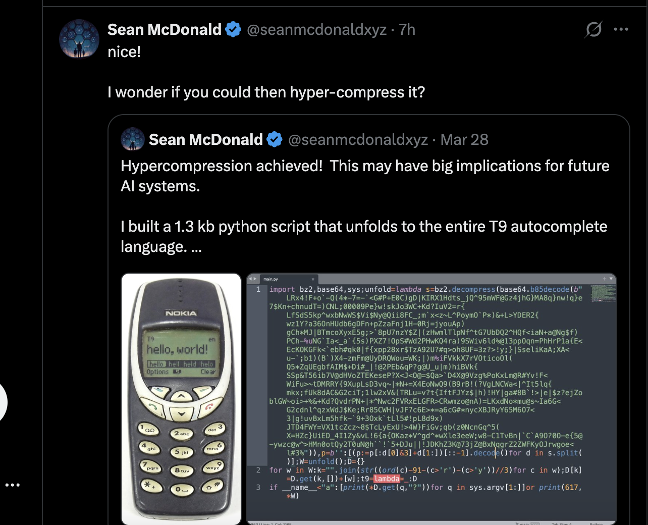
<p><img src="/images/amx-tweet-hypercompression.png" alt="Sean McDonald asking about hyper-compression" /></p>

<p><img src="/images/amx-tweet-where-to-start.png" alt="Elliot asking where to start" /></p>

<p>For anyone asking where to start: paste the paper into Claude Code. I’m not being glib. That is genuinely how a lot of this got built, and the paper was written to be reproducible from the configurations and logs released with it.</p>

<h2 id="on-working-with-claude">On working with Claude</h2>

<p>Several people asked how much of this was me and how much was the model. The paper names Claude Opus 5 as an author with its version string, rather than acknowledging “AI assistance,” because the version is what makes the claim checkable.</p>

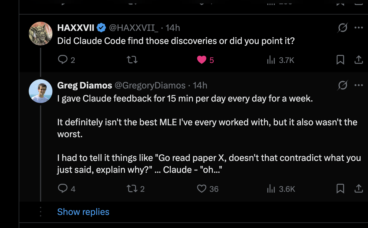
<p><img src="/images/amx-tweet-claude-discoveries.png" alt="A question about whether Claude Code found the discoveries" /></p>

<p>I gave Claude feedback for about 15 minutes a day for a week. It definitely isn’t the best MLE I’ve ever worked with, and it also wasn’t the worst. A lot of the work was me saying things like “go read paper X, doesn’t that contradict what you just said, explain why,” and getting back “oh…”</p>

<p><img src="/images/amx-tweet-abilities-in-data.png" alt="On disagreeing with Claude about what abilities should exist in the data" /></p>

<p>The most productive disagreement was about whether these abilities should exist in the data at all. Claude kept insisting the model was too small to learn X. I’d ask whether X appeared in the dataset. Yes. Then what happens if we isolate X — does it learn? “I can’t believe it did.”</p>

<p>That loop is where the results came from. Neither of us would have gotten there alone. It took a while for Claude to trust the experiments over its priors, but it eventually did — including the refutation in Section 8.3, where the ablation killed our own stated mechanism and we published the refutation next to the result.</p>

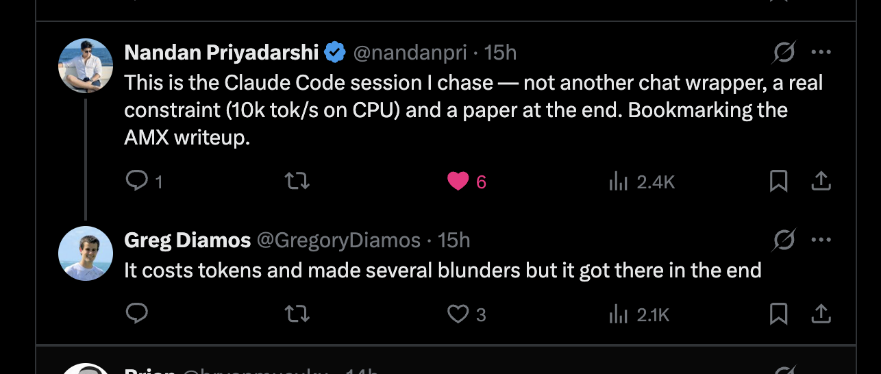
<p><img src="/images/amx-tweet-blunders.png" alt="On the token cost and blunders along the way" /></p>

<p>It cost tokens and made several blunders, but it got there in the end.</p>

<h2 id="the-title">The title</h2>

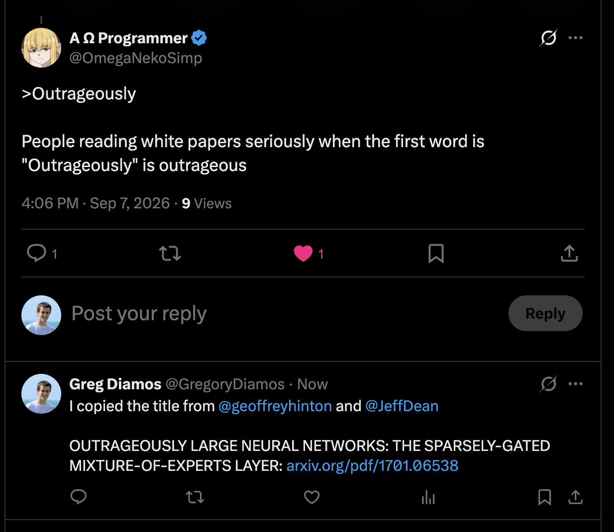
<p><img src="/images/amx-tweet-outrageously.png" alt="Someone objecting to the word &quot;Outrageously&quot;" /></p>

<p><img src="/images/amx-tweet-clickbait-title.png" alt="A comment about clickbait paper titles" /></p>

<p>I copied the title from Geoff Hinton and Jeff Dean. <a href="https://arxiv.org/pdf/1701.06538">Outrageously Large Neural Networks: The Sparsely-Gated Mixture-of-Experts Layer</a> is the paper that started all of this, and this work is the same idea pointed in the opposite direction. Clickbait titles are a tradition in ML and I’m not going to be the one who breaks it.</p>

<h2 id="why-this-post-exists">Why this post exists</h2>

<p><img src="/images/amx-tweet-blog-request.png" alt="Aamir suggesting the findings would read better as a blog post" /></p>

<p>Fair point. Here it is.</p>

<h2 id="what-id-want-someone-to-run-next">What I’d want someone to run next</h2>

<p>If you want to move this forward, in rough order of how cheap the experiment is against how much it would tell us:</p>

<ol>
  <li><strong>Hold the config fixed, re-run against newer corpus releases.</strong> If the distillation argument in Section 4 is right, capability on one core goes up every year with no change to the model. This is the cheapest experiment in the whole space and I think it’s the most likely source of near-term gains.</li>
  <li><strong>The equal-time comparison.</strong> Same wall clock instead of same tokens, dense against MoE. It could reverse my architecture conclusion, which is exactly why it should be run.</li>
  <li><strong>Somi’s control.</strong> The same recipe on plain pre-LLM web text, to separate curated corpus from capacity.</li>
  <li><strong>A frozen task and test set, multiple seeds, and a measured generation latency.</strong> stunspot’s agent listed this and it’s the right list.</li>
</ol>

<p>The claim here is not that this model is good. 18.2% exact match is weak by any contemporary standard, and 47% on two-digit addition is not a general calculation ability. The claim is that this much is reachable on one core, that it arrives much earlier than I assumed, and that the failures that remain are localized rather than diffuse.</p>

<p>The budget at which copying, positional manipulation and simple arithmetic become measurable is far lower than I thought, and it’s reachable on hardware cheap enough to leave running.</p>

<hr />

<ul>
  <li>Paper: <a href="https://huggingface.co/gdiamos/amx-reasoning-v1-instruct/blob/main/paper.pdf">Outrageously Small Neural Networks: Emergent Basic Reasoning at 6,616 tok/sec on One Intel AMX Core</a></li>
  <li>Model and code: <a href="https://huggingface.co/gdiamos/amx-reasoning-v1-instruct">gdiamos/amx-reasoning-v1-instruct</a></li>
  <li>The thread: <a href="https://x.com/GregoryDiamos/status/2096873745420075020">@GregoryDiamos</a></li>
</ul>]]></content><author><name>Greg Diamos</name></author><category term="Other" /><summary type="html"><![CDATA[I did not set out to write a paper about small models. I had a data processing problem.]]></summary></entry><entry><title type="html">LLM Decompression: Reverse-Engineering Models Into Datasets</title><link href="http://gregdiamos.com/2025/09/19/llm-deflate.html" rel="alternate" type="text/html" title="LLM Decompression: Reverse-Engineering Models Into Datasets" /><published>2025-09-19T00:00:00+00:00</published><updated>2025-09-19T00:00:00+00:00</updated><id>http://gregdiamos.com/2025/09/19/llm-deflate</id><content type="html" xml:base="http://gregdiamos.com/2025/09/19/llm-deflate.html"><![CDATA[<p>Large Language Models compress massive amounts of training data into their parameters. This compression is lossy but highly effective—billions of parameters can encode the essential patterns from terabytes of text. However, what’s less obvious is that this process can be reversed: we can systematically extract structured datasets from trained models that reflect their internal knowledge representation.</p>

<p>I’ve been working on this problem, and the results are promising. We’ve successfully applied this decompression technique to three popular open-source models and generated substantial training datasets from each.</p>

<h2 id="related-work">Related Work</h2>

<p>The concept of synthetic data generation for LLMs has evolved significantly from early experimental techniques to production-critical methodologies. This work builds on several key developments in the field.</p>

<h3 id="stanford-alpaca-and-self-instruction">Stanford Alpaca and Self-Instruction</h3>

<p>Stanford’s Alpaca dataset [1] demonstrated that high-quality instruction-following models could be created cost-effectively using synthetic data. The Alpaca team used text-davinci-003 to generate 52,000 instruction-following demonstrations through a self-instruct pipeline [2], starting with just 175 human-written seed examples. This approach showed that a 7B parameter model could achieve GPT-3.5-level performance for under $600 in training costs.</p>

<p>The key innovation was the iterative generation process: the model generates new instructions, creates responses, and uses successful examples for further training. This created a flywheel effect where synthetic data quality improved over successive iterations.</p>

<h3 id="nvidia-nemotron-data-generation-pipeline">NVIDIA Nemotron Data Generation Pipeline</h3>

<p>NVIDIA’s Nemotron-4 340B [3] represents the current state-of-the-art in industrial synthetic data generation. Their approach uses a sophisticated two-stage pipeline where over 98% of the model’s alignment training data is generated synthetically [4].</p>

<p>The system employs three specialized models: Nemotron-4-340B-Instruct for response generation, Nemotron-4-340B-Reward for quality evaluation, and the base model for foundation capabilities. The reward model evaluates responses across five dimensions (helpfulness, correctness, coherence, complexity, verbosity) using 0-4 Likert scales.</p>

<p>What makes Nemotron particularly impressive is the scale and quality control. The system generated over 100K synthetic conversations while maintaining strict quality standards through automated filtering and verification. This demonstrates that synthetic data generation can work at production scale with appropriate infrastructure.</p>

<h3 id="knowledge-distillation-and-model-decompression">Knowledge Distillation and Model Decompression</h3>

<p>Knowledge distillation techniques have evolved from simple output mimicking to sophisticated approaches that extract reasoning patterns and problem-solving strategies. Microsoft’s Orca [5] used GPT-4’s explanation traces to train smaller models, achieving significant performance improvements by learning from the reasoning process rather than just the final outputs.</p>

<p>Recent work in training data extraction [6] has shown that large language models memorize substantial portions of their training data. This suggests that the reverse process—systematic extraction of knowledge from trained models—should be feasible with the right techniques.</p>

<h2 id="the-technical-challenge">The Technical Challenge</h2>

<p>The core insight is straightforward: if an LLM has successfully compressed knowledge during training, we can use inference to decompress that knowledge back into structured data. The challenge is doing this systematically and at scale.</p>

<p>Traditional approaches to synthetic data generation are either too narrow (focusing on specific tasks) or too broad (generating random examples). What we need is a method that:</p>

<ol>
  <li>Systematically explores the model’s knowledge space</li>
  <li>Extracts both factual knowledge and reasoning patterns</li>
  <li>Scales efficiently with available inference compute</li>
  <li>Produces structured, reusable training data</li>
</ol>

<h2 id="implementation-details">Implementation Details</h2>

<p>The approach I’ve developed uses hierarchical topic exploration to systematically traverse a model’s knowledge space:</p>

<pre><code class="language-python">class TopicExplorer:
    def _expand_topic_tree(self):
        predecessors = self._get_predecessor_batch()
        new_topics = generate_new_topics(predecessors, seed=len(self.topic_tree))
        self.topic_tree.extend(new_topics)
</code></pre>

<p>Starting with broad categories, the system recursively generates more specific subtopics. This creates a tree structure that maps to how the model organizes domain knowledge internally.</p>

<p>For each topic node, we generate multiple training examples that capture both the model’s factual knowledge and its reasoning approach:</p>

<pre><code class="language-python">def make_question_prompt(topic, seed):
    prompt += "Your task is to write a challenging task and response that requires deep understanding of the topic.\n"
    prompt += "Think step by step.\n"
</code></pre>

<p>The key is asking for explicit reasoning steps. This extracts not just what the model knows, but how it approaches problems in that domain.</p>

<h2 id="scaling-considerations">Scaling Considerations</h2>

<p>The bottleneck in this process is inference cost. Generating comprehensive datasets requires thousands of model calls per topic, which quickly becomes expensive with traditional inference setups.</p>

<p>This is where scalarlm becomes essential. High-performance inference infrastructure allows us to:</p>

<ul>
  <li>Generate training examples in parallel across topic branches</li>
  <li>Iterate rapidly on prompt engineering and filtering logic</li>
  <li>Scale to comprehensive coverage of the model’s knowledge space</li>
  <li>Make the economics work for large-scale dataset generation</li>
</ul>

<p>Without efficient inference, this approach remains a research curiosity. With it, we can generate production-quality training datasets.</p>

<h2 id="results-and-datasets">Results and Datasets</h2>

<p>We’ve applied this methodology to three prominent open-source models:</p>

<ul>
  <li><strong>Qwen2.5-Coder</strong>: Specialized for code generation and programming tasks</li>
  <li><strong>GPT-OSS</strong>: General-purpose language model</li>
  <li><strong>NVIDIA Nemotron</strong>: Optimized for reasoning and instruction-following</li>
</ul>

<p>Each decompression run generated 10,000+ structured training examples covering the breadth of the model’s capabilities. The extracted datasets reveal interesting differences in how each model organizes and approaches different types of problems.</p>

<p><strong>Dataset samples are available on HuggingFace:</strong></p>
<ul>
  <li><a href="https://huggingface.co/datasets/masint/qwen3-30b-a3b-instruct-deflate-general">Qwen3-30B-A3B-Coder Decompressed Dataset</a></li>
  <li><a href="https://huggingface.co/datasets/masint/gpt-oss-deflate-general">GPT-OSS Decompressed Dataset</a></li>
  <li><a href="https://huggingface.co/datasets/masint/NVIDIA-Nemotron-Nano-12B-v2-deflate-general">Nemotron Decompressed Dataset</a></li>
</ul>

<h2 id="practical-applications">Practical Applications</h2>

<p>The extracted datasets have several immediate uses:</p>

<p><strong>Model Analysis</strong>: By examining the topics and reasoning patterns that emerge, we can systematically evaluate model capabilities across different domains. This is more comprehensive than traditional benchmark evaluations.</p>

<p><strong>Knowledge Transfer</strong>: The structured datasets can be used to fine-tune other models, effectively transferring knowledge from the source model. This is particularly useful for creating specialized models from general-purpose ones.</p>

<p><strong>Training Data Augmentation</strong>: For domains where training data is scarce, these synthetic examples can supplement existing datasets. The quality is often higher than naive data augmentation techniques.</p>

<p><strong>Model Debugging</strong>: When a model performs poorly on specific tasks, examining its decompressed knowledge in that area can reveal gaps or misconceptions in its training.</p>

<h2 id="technical-challenges-and-solutions">Technical Challenges and Solutions</h2>

<p>Several technical issues emerged during implementation:</p>

<p><strong>Prompt Engineering</strong>: Getting consistent, parseable output required careful prompt design. The system needs to reliably extract JSON-formatted training examples from free-form model responses.</p>

<p><strong>Topic Tree Balance</strong>: The hierarchical exploration can become unbalanced, over-sampling some areas while missing others. We addressed this with configurable expansion factors and batch processing.</p>

<p><strong>Quality Filtering</strong>: Not all generated examples are high quality. We implemented parsing validation and can add semantic filtering as needed.</p>

<p><strong>Computational Efficiency</strong>: Even with fast inference, generating comprehensive datasets takes substantial compute. We optimized batch processing and parallel generation to minimize costs.</p>

<h2 id="looking-forward">Looking Forward</h2>

<p>This decompression approach opens several research directions:</p>

<p><strong>Cross-Model Knowledge Transfer</strong>: Can we use datasets extracted from one model to improve another? Early experiments suggest this works, but more systematic evaluation is needed.</p>

<p><strong>Knowledge Evolution Tracking</strong>: As models are updated, we can decompress new versions and diff the resulting datasets to understand how their knowledge has changed.</p>

<p><strong>Specialized Dataset Creation</strong>: For domains where training data is expensive to create (like specialized technical fields), model decompression might be more cost-effective than human annotation.</p>

<p><strong>Model Interpretability</strong>: Large-scale decompression could help us understand how different models organize knowledge differently, providing insights into training methodology effectiveness.</p>

<h2 id="conclusion">Conclusion</h2>

<p>LLM decompression isn’t a silver bullet, but it’s a practical technique for systematically extracting value from trained models. The key insight is treating inference as a knowledge extraction tool rather than just a generation mechanism.</p>

<p>With efficient inference infrastructure, we can reverse-engineer the compressed knowledge in any model and convert it into structured, reusable datasets. This has immediate applications in model analysis, knowledge transfer, and training data creation.</p>

<p>The three datasets we’ve published demonstrate this approach works across different model architectures and specializations. As inference costs continue to decrease, I expect this type of systematic knowledge extraction to become a standard part of the ML toolkit.</p>

<p>The code is straightforward, the results are measurable, and the applications are practical. Sometimes the best solutions are the obvious ones executed well.</p>

<p><em>What knowledge might be hiding in your models, waiting to be decompressed?</em></p>

<h2 id="bibliography">Bibliography</h2>

<p>[1] Taori, R., Gulrajani, I., Zhang, T., Dubois, Y., Li, X., Guestrin, C., … &amp; Hashimoto, T. B. (2023). Stanford Alpaca: An instruction-following LLaMA model. Stanford Center for Research on Foundation Models.</p>

<p>[2] Wang, Y., Kordi, Y., Mishra, S., Liu, A., Smith, N. A., Khashabi, D., &amp; Hajishirzi, H. (2022). Self-Instruct: Aligning Language Models with Self-Generated Instructions. arXiv preprint arXiv:2212.10560.</p>

<p>[3] Parmar, M., Iyer, S., Ananthaswamy, A., Bubeck, S., &amp; Chen, W. (2024). Nemotron-4 340B Technical Report. arXiv preprint arXiv:2406.11704.</p>

<p>[4] NVIDIA Developer Blog. (2024). Leverage the Latest Open Models for Synthetic Data Generation with NVIDIA Nemotron-4-340B. NVIDIA Technical Blog.</p>

<p>[5] Mukherjee, S., Mitra, A., Jawahar, G., Agarwal, S., Palangi, H., &amp; Awadallah, A. (2023). Orca: Progressive Learning from Complex Explanation Traces of GPT-4. arXiv preprint arXiv:2306.02707.</p>

<p>[6] Carlini, N., Tramer, F., Wallace, E., Jagielski, M., Herbert-Voss, A., Lee, K., … &amp; Raffel, C. (2021). Extracting Training Data from Large Language Models. USENIX Security Symposium.</p>]]></content><author><name>Greg Diamos</name></author><category term="Other" /><summary type="html"><![CDATA[Large Language Models compress massive amounts of training data into their parameters. This compression is lossy but highly effective—billions of parameters can encode the essential patterns from terabytes of text. However, what’s less obvious is that this process can be reversed: we can systematically extract structured datasets from trained models that reflect their internal knowledge representation.]]></summary></entry><entry><title type="html">ScalarLM Benchmarking MI300X BF16 GEMM</title><link href="http://gregdiamos.com/2025/05/31/mi300x-bf16-gemm.html" rel="alternate" type="text/html" title="ScalarLM Benchmarking MI300X BF16 GEMM" /><published>2025-05-31T00:00:00+00:00</published><updated>2025-05-31T00:00:00+00:00</updated><id>http://gregdiamos.com/2025/05/31/mi300x-bf16-gemm</id><content type="html" xml:base="http://gregdiamos.com/2025/05/31/mi300x-bf16-gemm.html"><![CDATA[<p>This blog covers the performance of the MI300X GPU in the context of a bfloat16 GEMM benchmark.</p>

<p>Here are the specs of the MI300X GPU for reference:</p>

<ul>
  <li><strong>BF16 Compute</strong>: 1.3 PFLOP/s</li>
  <li><strong>FP8 Compute</strong>: 2.6 PFLOP/s</li>
  <li><strong>HBM</strong>: 192GB HBM3E</li>
  <li><strong>HBM Bandwidth</strong>: 5.3 TB/s</li>
  <li><strong>Power Consumption</strong>: 750W</li>
</ul>

<p>GEMM (General Matrix Multiply) is a fundamental operation in many machine learning and
scientific computing applications, particularly in training and inference of large
language models (LLMs). The MI300X GPU’s support for bfloat16 (BF16) precision allows
for efficient computation while maintaining a balance between performance and numerical
stability.</p>

<h2 id="gemm-on-mi300x">GEMM on MI300X</h2>

<p>MI300X has a bfloat16 flops to memory ratio of 2.6 PFLOP/s / 5.3 TB/s = 490 flops/bytes.
This means that for every byte of memory accessed, the MI300X needs to perform at least
490 floating point operations to achieve peak performance. In the context of a GEMM
operation, this means that each matrix dimension should be at least 490. While training
transformer LLMs, this ratio is typically achieved by batching over the sequence length.
However, during inference using auto-regressive decoding when one token is generated
per step, the sequence length is typically 1, which means that the batch size
must be large enough (i.e. more than 490) to achieve the required flops to memory ratio.
As we will see in the benchmark results, the compute to memory ratio typically needs
to be even higher than 490 due to the overhead of the GEMM operation itself.</p>

<p><img src="/images/mi300x-cdna-architecture.png" alt="CDNA GPU Architecture" /></p>

<p>Matrix multiplication in the MI300X GPU is performed by mapping the GEMM operation to the
CDNA architecture, which is composed of multiple compute units (CUs) that work in parallel.
The matrix multiplication is divided into smaller tiles, which are then processed by the CUs.
The core operation performed by each CU is a Matrix fused-multiply-add (MFMA) operation,
which computes the product of two matrices and adds the result to a third matrix, each
of which is stored in the CU’s register file. The V_MFMA_F32_BF16_BF16 instruction
performs a matrix multiplication of two bfloat16 matrices and accumulates the result
into a float32 matrix.</p>

<p><img src="/images/mi300x-chiplet.png" alt="CDNA Chiplet Architecture" /></p>

<p>The MI300X GPU is composed of 4 CDNA chiplets, each of which contains 76 CUs, each of
whcih containers 4 matrix cores. The chiplets are connected to each other using
Infinity Fabric links. The chiplets are connected to 2 HBM3 stacks each, creating
NUMA (Non-Uniform Memory Access) regions.</p>

<h2 id="bfloat16-format">Bfloat16 Format</h2>

<p>Bfloat16 is a 16-bit floating point format that is designed to provide a good balance
between performance and numerical stability. It has the same exponent range as
float32, but only 7 bits of precision in the mantissa. This means that it can represent
a wide range of values, but with less precision than float32. The bfloat16 format is
commonly used in deep learning applications, particularly for training and inference of
large language models (LLMs). It allows for efficient computation while maintaining
numerical stability, as the exponent range is sufficient to represent the values
typically encountered in deep learning workloads.</p>

<p><img src="/images/bfloat16.png" alt="Bfloat16 Format" /></p>

<p>The exponent is stored in 8 bits, with the lowest representable value being
-126 and the highest representable value being 127. Accumulation is performed in
float32, which allows for higher precision in the final result. During mixed precision
training, the weights and input activations are typically cast to bfloat16 before
performing the GEMM operation. In particular, a common value of 1.0f corresponds to
an exponent of 127 in bfloat16, or in hex 0x7f00, where all bits of the exponent are
set to 1.</p>

<h2 id="benchmark-results">Benchmark Results</h2>

<p><img src="/images/mi300x-gemm.png" alt="GEMM Benchmark" /></p>

<p>The benchmark results show that the MI300X achieves a peak performance of 890 TFLOP/s
for bfloat16 GEMM operations, which is 68.4% of the theoretical peak performance of 1.3 PFLOP/s.
MI300X has a power limit of 750W, which becomes the limiting factor for the performance
of compute intensive operations like GEMM.</p>

<p><img src="/images/mi300x-power-and-clocks.png" alt="GEMM Power and Clocks" /></p>

<p>The power consumption of the MI300X during the benchmark is maxed out at 750W. During
the most power intensive benchmark, with a large GEMM operation with random bits,
the CU clocks are scaled down to 1.1 GHz to stay within the power limit.</p>

<p>Best performance is achieved with a compute intensity of 1365 flops/byte for square
4k by 4k matrices, which is significantly higher than the theoretical minimum of 490 flops/byte.</p>

<h2 id="the-number-of-zeros-matters">The number of zeros matters</h2>

<p><img src="/images/mi300x-gemm-zero-bits.png" alt="GEMM Benchmark" /></p>

<p>In this figure we sweep the number of zero bits in the input matrices to see how it
affects the performance of the GEMM operation. If the inputs are random normally distributed,
the performance is 645 TFLOP/s. If the inputs are all zeros, the performance in increases
to 890 TFLOP/s. Importantly, for common values from a function like torch.randn
with magnitudes between 0.1f and 1.0f, the exponent has 6 or 7 bits set to one because the
exponent is stored in two’s complement format. If we scale the numbers down by a factor of
2^-119, we can cut the average number of exponents bits set to one down to 2. This results in a
performance of 780 TFLOP/s. This suggests that a huge speedup of 1.37x is possible by
paying close attention to the distribution of weight, activation, and delta values in the
input matrices.</p>

<h2 id="analysis">Analysis</h2>

<p>Most practical workloads, especially inference scenarios with small batch sizes, operate
in the steep memory-bound region where performance scales linearly with operational intensity.
The data points clustering around 10-100 FLOP/byte represent typical LLM inference scenarios,
where the MI300X delivers only 5-100 TFLOP/s—far below its theoretical peak. This suggests
that batching is incredibly important for achieving high inference performance on the MI300X,
especially for requests with large numbers of output tokens.</p>

<h2 id="pytorch-benchmark-code">PyTorch Benchmark Code</h2>

<p>You can find the benchmark code on the <a href="https://github.com/tensorwavecloud/ScalarLM/blob/main/test/benchmark/pytorch/gemm.py">ScalarLM GEMM Github</a>.</p>

<p>Let’s take a look at the code:</p>

<h3 id="gemm-sizes">GEMM Sizes</h3>

<pre><code class="language-python">llama_8b_sizes = [
    (1, 4096, 4096),
    (2, 4096, 4096),
    (4, 4096, 4096),
    (8, 4096, 4096),
    (16, 4096, 4096),
    (32, 4096, 4096),
    (64, 4096, 4096),
    (128, 4096, 4096),
    (256, 4096, 4096),
    (512, 4096, 4096),
    (1024, 4096, 4096),
    (2048, 4096, 4096),
    (4096, 4096, 4096),
    (4096, 4096, 2048),
    (128256, 4096, 2048),
    (2048, 4096, 14336),
    (16384, 16384, 16384),
]
</code></pre>

<p>This code sets up the sizes of the GEMM operations to be benchmarked. The sizes are tuples of the form
<code>(m, n, k)</code>, where <code>m</code> is the number of rows in the first matrix, <code>n</code> is the number of columns in the second matrix,
and <code>k</code> is the number of columns in the first matrix (or rows in the second matrix). The sizes are chosen to be
representative of the sizes of the matrices used in the Llama 3 8B model. The sizes range from small matrices
(1x4096) to large matrices (4096x4096), with some intermediate sizes. The largest size is 128256x4096, which is
the size of the embedding table in the Llama 3 8B model. The sizes are chosen to be powers of 2, which is a common
practice in deep learning to optimize memory access patterns and performance on GPUs.</p>

<h3 id="benchmark-setup">Benchmark Setup</h3>

<p>Next, we set up the benchmark:</p>

<pre><code class="language-python">def run_gemm_benchmark():
    warmup()

    results = {}

    for size in tqdm(gemm_sizes):
        results[str(size)] = run_gemm(size)

    return results
</code></pre>

<p>This function runs the GEMM benchmark. It first warms up the GPU by running a few iterations of the GEMM kernel
without measuring the time. This is done to ensure that the GPU is in a good state before running the benchmark. The
function then runs the GEMM kernel for each size in the <code>gemm_sizes</code> list and measures the time taken to perform the
GEMM operation.</p>

<h3 id="warmup">Warmup</h3>

<p>Warmup is pretty simple.</p>

<pre><code class="language-python">def warmup():
    run_gemm((256, 256, 2048))

    global gemm_sizes
    gemm_sizes = select_appropriate_size_for_this_machine()

</code></pre>

<p>This function runs the GEMM kernel with a size of 256x256x2048 to warm up the GPU. This is a small size that is
sufficient to warm up the GPU without taking too long. The function also sets the <code>gemm_sizes</code> variable to the
appropriate sizes for the current machine. The <code>select_appropriate_size_for_this_machine</code> function is used to
select the appropriate sizes based on how long it takes to run.</p>

<h3 id="running-gemm-pytorch">Running GEMM PyTorch</h3>

<p>The <code>run_gemm</code> function is where the actual GEMM kernel is run. It uses PyTorch to allocate memory on the GPU and
perform the matrix multiplication. The function measures the time taken to perform the GEMM operation and calculates
the performance metrics such as FLOPS, bytes transferred, and operational intensity.</p>

<p>The function uses PyTorch’s <code>matmul</code> method to perform the matrix multiplication. The <code>out</code> parameter is used to specify
the output tensor where the result of the multiplication will be stored. This is more efficient than creating a new tensor
for the result because it avoids allocating memory for the result tensor. The function also uses PyTorch’s CUDA events
to measure the time taken to execute the kernel. CUDA events are used to measure the time taken to execute a kernel on
the GPU. The <code>record</code> method is used to record the time at which the event is recorded, and the <code>elapsed_time</code> method
is used to calculate the time taken to execute the kernel. The time is measured in milliseconds, so we multiply by
1e-3 to convert to seconds. Using events is necessary because the GPU is asynchronous, meaning that the CPU and GPU can
run in parallel. The CPU can continue executing while the GPU is performing the matrix multiplication. This can lead to
misleading results if the time taken to execute the kernel is not measured correctly.</p>

<pre><code class="language-python">def run_gemm(size):
    m, n, k = size
    #a = torch.randint(0, 1, (m, k), dtype=gemm_dtype, device=get_device())
    #b = torch.randn(k, n, dtype=gemm_dtype, device=get_device()) * torch.randint(0, 1, (k, n), dtype=gemm_dtype, device=get_device())
    #b = torch.randint(0, 1, (k, n), dtype=gemm_dtype, device=get_device())
    a = make_random(m, k, 8, 8, 2**-119)  #torch.randn(m, k, dtype=gemm_dtype, device=get_device())
    b = make_random(n, k, 8, 8, 2**-119)  #torch.randn(n, k, dtype=gemm_dtype, device=get_device())
    c = torch.zeros(m, n, dtype=gemm_dtype, device=get_device())

    # run at least 3 seconds
    start_time = time.time()
    end_time = start_time + 3

    barrier()

    start = get_event()
    end = get_event()

    start.record()
    iterations = 0
    while time.time() &lt; end_time:
        torch.matmul(a, b.T, out=c)
        iterations += 1
    end.record()

    iterations = max(1, iterations)

    barrier()

    seconds = start.elapsed_time(end) / 1000 / iterations

    return {
        "size": size,
        "time": seconds,
        "flops": 2 * m * n * k,
        "flop/s": 2 * m * n * k / seconds,
        "bytes": (m * k + k * n + m * n) * 2,
        "operational_intensity": 2 * m * n * k / ((m * k + k * n + m * n) * 2),
        "GFLOP/s": 2 * m * n * k / seconds / 1e9,
    }
</code></pre>

<h3 id="handling-gpus">Handling GPUs</h3>

<p>When running on a GPU, the benchmark uses PyTorch’s CUDA events to measure the time taken to copy the data. CUDA events are
used to measure the time taken to execute a kernel on the GPU. The <code>record</code> method is used to record the time at which
the event is recorded. The <code>elapsed_time</code> method is used to calculate the time taken to execute the kernel. The time
is measured in milliseconds, so we multiply by 1e-3 to convert to seconds. Using events is necessary because the GPU
is asynchronous, meaning that the CPU and GPU can run in parallel. The CPU can continue executing while the GPU is
copying data. This can lead to misleading results if the time taken to copy the data is not measured correctly.</p>

<p>In order to make the code cross-platform, we define a <code>get_event</code> function that returns a CUDA event if the GPU is available, or a CPU event
if the GPU is not available. The CPU event is a simple wrapper around the time module that records the time when the event is created and
calculates the elapsed time between two events.</p>

<pre><code class="language-python">class CPUEvent:
    def __init__(self):
        self.time = 0

    def record(self):
        self.time = time.time()

    def elapsed_time(self, other):
        return (other.time - self.time) * 1000


def get_event():
    if torch.cuda.is_available():
        return torch.cuda.Event(enable_timing=True)
    else:
        return CPUEvent()


def barrier():
    if torch.cuda.is_available():
        torch.cuda.synchronize()
    else:
        pass

def get_device():
    if torch.cuda.is_available():
        return torch.device("cuda:0")
    else:
        return torch.device("cpu")
</code></pre>

<h2 id="selecting-the-appropriate-size-for-the-machine">Selecting the appropriate size for the machine</h2>

<p>The <code>select_appropriate_size_for_this_machine</code> function is used to select the appropriate sizes for the GEMM operations
based on the performance of a small GEMM operation. The function runs a small GEMM operation with a size of 256x256x2048
and measures the time taken to perform the operation. It then calculates the performance metrics such as FLOPS, bytes transferred,
and operational intensity. The function then calculates the time it would take to run each of the Llama model sizes based
on the performance of the small GEMM operation.</p>

<pre><code class="language-python">def select_appropriate_size_for_this_machine():
    # Try a small GEMM, and time it
    # If it runs too fast, select a bigger model
    # If it runs too slow, select a smaller model
    tiny_gemm = (256, 256, 2048)

    metrics = run_gemm(tiny_gemm)

    # Get the total number of flops in each model

    def get_flops(size):
        m, n, k = size
        return 2 * m * n * k

    tiny_flops = get_flops(tiny_gemm)

    logger.info(f"Tiny GEMM took {metrics['time']} seconds it ran at {metrics['GFLOP/s']} GFLOP/s")

    # get the flops for each llama model
    llama_100m_flops = sum([get_flops(size) for size in llama_100m_sizes])
    llama_1b_flops = sum([get_flops(size) for size in llama_1b_sizes])
    llama_8b_flops = sum([get_flops(size) for size in llama_8b_sizes])

    # Get the time it took to run the tiny gemm
    tiny_time = metrics["time"]

    # Get the time it would take to run each llama model
    llama_100m_time = llama_100m_flops / tiny_flops * tiny_time
    llama_1b_time = llama_1b_flops / tiny_flops * tiny_time
    llama_8b_time = llama_8b_flops / tiny_flops * tiny_time

    logger.info(f"GEMM from llama_100m will take {llama_100m_time} seconds")
    logger.info(f"GEMM from llama_1b will take {llama_1b_time} seconds")
    logger.info(f"GEMM from llama_8b will take {llama_8b_time} seconds")

    # Select the largest model that will take at most 10 seconds to run
    if llama_8b_time &lt; 10:
        return llama_8b_sizes
    elif llama_1b_time &lt; 10:
        return llama_1b_sizes
    elif llama_100m_time &lt; 10:
        return llama_100m_sizes
    else:
        return [tiny_gemm]
</code></pre>]]></content><author><name>Greg Diamos</name></author><category term="Other" /><summary type="html"><![CDATA[This blog covers the performance of the MI300X GPU in the context of a bfloat16 GEMM benchmark.]]></summary></entry><entry><title type="html">ScalarLM Benchmarking MI300X Memcpy Peer</title><link href="http://gregdiamos.com/2025/05/08/mi300x-benchmark-memcpy-peer.html" rel="alternate" type="text/html" title="ScalarLM Benchmarking MI300X Memcpy Peer" /><published>2025-05-08T00:00:00+00:00</published><updated>2025-05-08T00:00:00+00:00</updated><id>http://gregdiamos.com/2025/05/08/mi300x-benchmark-memcpy-peer</id><content type="html" xml:base="http://gregdiamos.com/2025/05/08/mi300x-benchmark-memcpy-peer.html"><![CDATA[<p>This blog covers the performance of the MI300X GPU in the context of a memcpy peer benchmark.</p>

<p>Here are the specs of the MI300X GPU for reference:</p>

<ul>
  <li><strong>HBM</strong>: 192GB HBM3E</li>
  <li><strong>HBM Bandwidth</strong>: 5.3 TB/s</li>
  <li><strong>Infinity Fabric Link Bandwidth</strong>: 50 GB/s</li>
  <li><strong>Infinity Fabric Links Per GPU</strong>: 7</li>
  <li><strong>BF16 Compute</strong>: 1.3 PFLOP/s</li>
  <li><strong>FP8 Compute</strong>: 2.6 PFLOP/s</li>
</ul>

<p>Memcpy peer is used to measure the memory bandwidth when copying data between two
different GPUs on the same node. Memcpy peer is a good indicator of collective
operations such as all-reduce, all-gather, and scatter-reduce. Collective operations
are used to distribute LLMs across multiple GPUs. The performance of these operations is
critical for training and inference of large language models.</p>

<h2 id="mi300x-intra-node-network-architecture">MI300X Intra-Node Network Architecture</h2>

<p><img src="/images/mi300x-infinity-links.png" alt="Memcpy Peer Benchmark" /></p>

<p>Looking at the diagram, we can see eight MI300X DAMs (Discrete Accelerator Modules) arranged in an octagonal configuration, interconnected via AMD’s Infinity Fabric. The red lines illustrate the direct GPU-to-GPU Infinity Fabric links, forming a fully connected mesh topology where each GPU maintains direct connections to all other GPUs in the system. This design eliminates multi-hop communication paths, allowing any GPU to communicate with any other GPU through a single direct link with the full 50 GB/s bandwidth per link.</p>

<p>This architecture significantly enhances GPU-to-GPU peer performance for memory transfers. With each GPU having a direct 50 GB/s Infinity Fabric link to every other GPU, memcpy peer operations—which directly impact collective operations like all-reduce, all-gather, and scatter-reduce—can achieve optimal performance. The fully connected topology minimizes latency by eliminating the need for data to traverse through intermediate GPUs or the CPU, which would otherwise create bottlenecks in collective operations. This is particularly crucial for distributed training and inference of large language models where frequent synchronization between GPUs is required.</p>

<h2 id="benchmark-results">Benchmark Results</h2>

<p>This figure plots memcpy peer bandwidth against the size of the data being copied.
The x-axis is the size of the data being copied in bytes, and the y-axis is the bandwidth in GB/s.</p>

<p>The data is copied from one location in one GPU’s memory to another location in another GPU’s memory.
We use PyTorch to show the performance of the memcpyPeer API. We also show GPU-aware MPI_Send
and MPI_Recv for comparison.</p>

<p>The benchmark is run for different sizes of data, ranging from 4KB to 2.1GB, which is the size
of the embedding tables in the Llama 3.1 8B model.</p>

<h2 id="pytorch-memcpy-peer-benchmark">PyTorch Memcpy Peer Benchmark</h2>

<p><img src="/images/mi300x-memcpy-peer-benchmark.png" alt="Memcpy Peer Benchmark" /></p>

<p>The benchmark results for the AMD MI300X MemcpyPeer bandwidth demonstrate clear scaling patterns across different data transfer sizes. As shown in the logarithmic plot, the achieved bandwidth starts at just a few GB/s for very small transfers (below 100KB) and gradually increases with data size until reaching the theoretical maximum of 50 GB/s (marked as the “Roofline” on the graph) at approximately the 8-16MB range. This scaling behavior illustrates the classic relationship between data transfer size and bandwidth utilization, where small transfers are dominated by fixed overheads while larger transfers can more effectively saturate the available bandwidth.</p>

<p>The results reveal that the MI300X Infinity Fabric links reach near-optimal performance (above 40 GB/s) once transfer sizes exceed approximately 8MB, with the bandwidth curve flattening as it approaches the 50 GB/s roofline. This indicates that the communication protocol and hardware implementation have been well-optimized to minimize overhead for large data transfers. The bandwidth stabilizes completely for transfers larger than 32MB, suggesting that at this point, the system fully leverages the available bandwidth of the Infinity Fabric link without additional scaling benefits from increasing the data size further.</p>

<p>Most notably, the bandwidth curve shows a dramatic improvement between 100KB and 10MB data sizes, where performance increases from approximately 10-15 GB/s to over 40 GB/s. This critical transition zone represents an important threshold for application developers and system architects, as it determines the minimum message size needed to achieve efficient communication between MI300X GPUs. Understanding this threshold is essential for optimizing collective operations in distributed AI workloads, where the granularity of data partitioning can significantly impact overall system performance.</p>

<p>Key Learnings:</p>

<ul>
  <li>Bandwidth Saturation Point: The MI300X Infinity Fabric links reach approximately 90% of theoretical bandwidth at 8-16MB transfer sizes, indicating the minimum message size for optimal communication efficiency.</li>
  <li>Small Transfer Penalty: For data transfers smaller than 1MB, bandwidth utilization drops significantly, with 100KB transfers achieving only about 20% of peak bandwidth. This suggests a need for message aggregation strategies in applications dealing with small data blocks.</li>
  <li>Near-Linear Scaling Region: The log-log plot reveals a near-linear scaling region between 100KB and 8MB, where each doubling of message size yields substantial bandwidth improvements, making this range particularly sensitive to optimization efforts.</li>
  <li>Protocol Efficiency: The ability to achieve very close to the theoretical 50 GB/s limit demonstrates excellent protocol efficiency with minimal overhead for large transfers, indicating well-designed hardware and driver implementations.</li>
  <li>Implications for AI Workloads: For distributed training of large language models, these results suggest that tensor partitioning strategies should aim for partition sizes of at least 16MB to ensure optimal GPU-to-GPU communication performance across the Infinity Fabric interconnect.</li>
</ul>

<p>The performance characteristics demonstrated in these benchmarks validate AMD’s fully connected topology approach for the MI300X platform. The ability to consistently achieve near-theoretical bandwidth between directly connected GPUs confirms that the direct GPU-to-GPU links can effectively eliminate communication bottlenecks in multi-GPU configurations, provided that applications are structured to leverage appropriate transfer sizes. For HPC and AI system architects, these results highlight the importance of data partitioning strategies that maximize message sizes while maintaining computational efficiency across the distributed system.</p>

<h2 id="mpi-memcpy-peer-benchmark">MPI Memcpy Peer Benchmark</h2>

<p><img src="/images/mi300x-memcpy-peer-mpi-benchmark.png" alt="Memcpy Peer Benchmark" /></p>

<p>This benchmark demonstrates the bandwidth performance of AMD’s MI300X GPU using MPI_Send and MPI_Recv operations across a 50 GB/s Infinity Fabric link. The data reveals several important performance characteristics that would be relevant to HPC system architects.</p>

<p>The graph shows a clear bandwidth saturation pattern. For small data transfers (below 10MB), the achieved bandwidth is significantly lower than the theoretical maximum of 50 GB/s. However, as data size increases beyond 10MB, the bandwidth approaches and eventually reaches the theoretical roofline of 50 GB/s. This indicates that the MI300X requires larger message sizes to efficiently utilize the full bandwidth capacity of the Infinity link, which is typical of high-performance interconnects where protocol overhead dominates with smaller transfers.</p>

<p>What’s particularly notable is the steep bandwidth curve between 1-10MB message sizes, where performance rapidly improves from approximately 12 GB/s to nearly 40 GB/s. Beyond 16.8MB (represented by the green diamond), almost all data points cluster near the 50 GB/s roofline, showing that the system efficiently utilizes the available bandwidth for larger data transfers. The largest tested size of 1.1GB achieves essentially full utilization of the link.</p>

<p>Key Insights:</p>

<ul>
  <li>Bandwidth Saturation Point: The MI300X requires approximately 16.8MB message size to reach ~80% of theoretical bandwidth, and 33.6MB to achieve &gt;90% utilization of the Infinity link.</li>
  <li>Small Message Inefficiency: Transfers below 4.2MB achieve less than 50% of the theoretical bandwidth, with the smallest sizes (4.1kB) managing only about 4% utilization. This highlights the significant protocol overhead for small transfers.</li>
  <li>Logarithmic Scaling: The consistent improvement across logarithmic increases in data size suggests well-designed network protocols that efficiently handle varying workloads.</li>
  <li>Practical Performance Threshold: HPC applications should batch communications to exceed 16.8MB when possible to maximize bandwidth utilization on the MI300X.</li>
  <li>Interconnect Ceiling: The hard limit at 50 GB/s confirms that the single Infinity link is the bottleneck rather than the GPU memory subsystem, suggesting that multi-link configurations would be beneficial for bandwidth-sensitive applications.</li>
</ul>

<p>These benchmark results provide valuable guidance for HPC developers optimizing communication patterns on MI300X-based systems, particularly highlighting the importance of message size on achievable performance when using MPI point-to-point operations.</p>

<h2 id="pytorch-benchmark-code">PyTorch Benchmark Code</h2>

<p>You can find the benchmark code on the <a href="https://github.com/tensorwavecloud/ScalarLM/blob/main/test/benchmark/pytorch/memcpy_peer.py">ScalarLM Peer Memcpy Github</a>.</p>

<p>Let’s take a look at the code:</p>

<h3 id="memcpy-sizes">Memcpy Sizes</h3>

<pre><code class="language-python"># List of memcpy sizes, in bytes, should be multiples of the page size
# Go up to the tensor size used in Llama 3 (4096 * 128256 * 4) = 2_101_346_304
memcpy_sizes = [ 2 ** i for i in range(12, 64) if 2 ** i &lt;= 2_101_346_304 ]
</code></pre>

<p>This code sets up the sizes of the data to be copied. The sizes are powers of 2, starting from 4KB (2^12) and going up to
1.1GB (2^30). The sizes are chosen to be multiples of the page size, which is 4KB on most systems. The maximum size is
the size of the embedding tables in the Llama 3 8B model, which is 2_101_346_304 bytes (or 2.1GB). The benchmark is run for
each of these sizes, and the bandwidth is measured for each size. The results are plotted in the figure above.</p>

<h3 id="benchmark-setup">Benchmark Setup</h3>

<p>Next, we set up the benchmark:</p>

<pre><code class="language-python">def run_memcpy_benchmark():

    warmup()

    results = {}

    for size in tqdm(memcpy_sizes):
        results[size] = run_memcpy(size)

    return results
</code></pre>

<p>This function runs the memcpy benchmark. It first warms up the GPU by running a few iterations of the memcpy kernel
without measuring the time. This is done to ensure that the GPU is in a good state before running the benchmark. The
function then runs the memcpy kernel for each size in the <code>memcpy_sizes</code> list and measures the time taken to copy the data.</p>

<h3 id="warmup">Warmup</h3>

<p>Warmup is pretty simple.</p>

<pre><code class="language-python">def warmup():
    run_memcpy(4096)
</code></pre>

<p>This function runs the memcpy kernel with a size of 4KB (4096 bytes) to warm up the GPU. GPUs have startup times to
load the code, ramp up the clocks, etc. Running benchmarks without a warmup can lead to misleading results.</p>

<h3 id="running-memcpy-peer-pytorch">Running Memcpy Peer PyTorch</h3>

<p>The <code>run_memcpy</code> function is where the actual memcpy kernel is run. It uses PyTorch to allocate memory on the GPU and
copy data from one location to another. The function measures the time taken to copy the data and calculates the bandwidth
and other metrics.</p>

<p>The memcpy kernel is run for at least 1 second to get a good measurement of the bandwidth. The function uses PyTorch’s
<code>copy_</code> method to copy data from one tensor to another. copy_ is the in-place version of the copy method, which means
that it modifies the destination tensor in place. This is more efficient than creating a new tensor for the result because it avoids
allocating memory for the result tensor.</p>

<pre><code class="language-python">def run_memcpy(size):
    a = torch.zeros(size // 4, device=get_device(), dtype=torch.float32) # size is in bytes, so divide by 4 to get number of floats
    b = torch.zeros(size // 4, device=get_device(), dtype=torch.float32)

    # copy for at least 1 second
    barrier()

    start = get_event()
    end = get_event()

    start_time = time.time()

    start.record()
    iterations = 0
    while time.time() - start_time &lt; 1:
        b.copy_(a)
        iterations += 1
    end.record()

    barrier()
    total_time = start.elapsed_time(end) * 1e-3 / iterations

    return {
        "operational_intensity": 1 / 4,  # 1 FLOP per 4 bytes
        "flop/s": size / 4 / total_time,
        "bytes": size,
        "time": total_time,
        "iterations": iterations,
        "bandwidth": size / total_time,
        "GB/s": size / total_time / 1e9,
    }
</code></pre>

<h3 id="handling-gpus">Handling GPUs</h3>

<p>When running on a GPU, the benchmark uses PyTorch’s CUDA events to measure the time taken to copy the data. CUDA events are
used to measure the time taken to execute a kernel on the GPU. The <code>record</code> method is used to record the time at which
the event is recorded. The <code>elapsed_time</code> method is used to calculate the time taken to execute the kernel. The time
is measured in milliseconds, so we multiply by 1e-3 to convert to seconds. Using events is necessary because the GPU
is asynchronous, meaning that the CPU and GPU can run in parallel. The CPU can continue executing while the GPU is
copying data. This can lead to misleading results if the time taken to copy the data is not measured correctly.</p>

<p>In order to make the code cross-platform, we define a <code>get_event</code> function that returns a CUDA event if the GPU is available, or a CPU event
if the GPU is not available. The CPU event is a simple wrapper around the time module that records the time when the event is created and
calculates the elapsed time between two events.</p>

<pre><code class="language-python">class CPUEvent:
    def __init__(self):
        self.time = 0

    def record(self):
        self.time = time.time()

    def elapsed_time(self, other):
        return (other.time - self.time) * 1000


def get_event():
    if torch.cuda.is_available():
        return torch.cuda.Event(enable_timing=True)
    else:
        return CPUEvent()


def barrier():
    if torch.cuda.is_available():
        torch.cuda.synchronize()
    else:
        pass

def get_device():
    if torch.cuda.is_available():
        return torch.device("cuda:0")
    else:
        return torch.device("cpu")
</code></pre>

<h2 id="mpi-benchmark-code">MPI Benchmark Code</h2>

<p>You can find the MPI benchmark code on <a href="https://github.com/tensorwavecloud/ScalarLM/blob/main/test/infra/distribution_strategy/benchmark_mpi_sendrecv.py">Github</a>.</p>]]></content><author><name>Greg Diamos</name></author><category term="Other" /><summary type="html"><![CDATA[This blog covers the performance of the MI300X GPU in the context of a memcpy peer benchmark.]]></summary></entry><entry><title type="html">ScalarLM Benchmarking MI300X Memcpy</title><link href="http://gregdiamos.com/2025/04/25/mi300x-benchmark-memcpy.html" rel="alternate" type="text/html" title="ScalarLM Benchmarking MI300X Memcpy" /><published>2025-04-25T00:00:00+00:00</published><updated>2025-04-25T00:00:00+00:00</updated><id>http://gregdiamos.com/2025/04/25/mi300x-benchmark-memcpy</id><content type="html" xml:base="http://gregdiamos.com/2025/04/25/mi300x-benchmark-memcpy.html"><![CDATA[<p>This blog covers the performance of the MI300X GPU in the context of a memcpy benchmark.</p>

<p>Here are the specs of the MI300X GPU for reference:</p>

<ul>
  <li><strong>HBM</strong>: 192GB HBM3E</li>
  <li><strong>Bandwidth</strong>: 5.3 TB/s</li>
  <li><strong>BF16 Compute</strong>: 1.3 PFLOP/s</li>
  <li><strong>FP8 Compute</strong>: 2.6 PFLOP/s</li>
</ul>

<p>Memcpy is used to measure the memory bandwidth of the GPU. The benchmark is run using a
simple memcpy kernel that copies data from one location to another in the GPU’s memory.
Memcpy is a good indicator of memory bound kernels, which are common in the activation
functions of LLMs.</p>

<h2 id="benchmark-results">Benchmark Results</h2>

<p>This figure plots memcpy bandwidth against the size of the data being copied. The x-axis is the size of the
data being copied in bytes, and the y-axis is the bandwidth in GB/s. The data is copied from one location to another
in the GPU’s memory. The benchmark is run for different sizes of data, ranging from 4KB to 2.1GB, which is the size
of the embedding tables in the Llama 3 8B model.</p>

<p><img src="/images/mi300x-memcpy-benchmark.png" alt="Memcpy Benchmark" /></p>

<p>Looking at this graph showing the AMD Instinct MI300X memory bandwidth for different data sizes, let’s analyze what’s happening with the memcpy performance:
The graph plots memory bandwidth (GB/s) on the y-axis against data size (MB) on the x-axis, both on logarithmic scales. Here are the key observations:</p>

<ol>
  <li>Roofline Performance: There’s a horizontal dashed line at approximately 5300 GB/s labeled as “Roofline” - this represents the theoretical maximum memory bandwidth of the MI300X GPU.</li>
  <li>Bandwidth Scaling: The graph shows how memory bandwidth scales with data size:
    <ul>
      <li>For very small data sizes (below 1MB), the bandwidth is quite low (under 100 GB/s)</li>
      <li>As data size increases, bandwidth improves dramatically</li>
      <li>Performance peaks for data sizes around 10-100MB, approaching but not quite reaching the roofline</li>
    </ul>
  </li>
  <li>Performance Plateau: For data sizes larger than about 10MB, the bandwidth levels off at approximately 2000-3000 GB/s, which is about 40-60% of the theoretical maximum.</li>
  <li>Various Transfer Sizes: The different markers represent different copy sizes (from 4.1kB to 1.1GB), showing how each performs across the spectrum.</li>
  <li>Memory Hierarchy Effects: The shape of this curve is typical of memory systems with hierarchical caches:
    <ul>
      <li>Small transfers are limited by overhead and latency</li>
      <li>Medium-sized transfers achieve the best bandwidth utilization</li>
      <li>Very large transfers may be hitting memory management limitations</li>
    </ul>
  </li>
</ol>

<p>This benchmark reveals that while the MI300X offers impressive memory bandwidth, real-world memcpy operations in PyTorch achieve around half of the theoretical maximum, which is actually quite good for practical workloads. The performance characteristics suggest that for optimal memory throughput, data should be processed in chunks of approximately 10-100MB when possible.</p>

<h2 id="benchmark-code">Benchmark Code</h2>

<p>You can find the benchmark code on the <a href="https://github.com/tensorwavecloud/ScalarLM/blob/main/test/benchmark/pytorch/memcpy.py">ScalarLM Github</a>.</p>

<p>Let’s take a look at the code:</p>

<h3 id="memcpy-sizes">Memcpy Sizes</h3>

<pre><code class="language-python"># List of memcpy sizes, in bytes, should be multiples of the page size
# Go up to the tensor size used in Llama 3 (4096 * 128256 * 4) = 2_101_346_304
memcpy_sizes = [ 2 ** i for i in range(12, 64) if 2 ** i &lt;= 2_101_346_304 ]
</code></pre>

<p>This code sets up the sizes of the data to be copied. The sizes are powers of 2, starting from 4KB (2^12) and going up to
1.1GB (2^30). The sizes are chosen to be multiples of the page size, which is 4KB on most systems. The maximum size is
the size of the embedding tables in the Llama 3 8B model, which is 2_101_346_304 bytes (or 2.1GB). The benchmark is run for
each of these sizes, and the bandwidth is measured for each size. The results are plotted in the figure above.</p>

<h3 id="benchmark-setup">Benchmark Setup</h3>

<p>Next, we set up the benchmark:</p>

<pre><code class="language-python">def run_memcpy_benchmark():

    warmup()

    results = {}

    for size in tqdm(memcpy_sizes):
        results[size] = run_memcpy(size)

    return results
</code></pre>

<p>This function runs the memcpy benchmark. It first warms up the GPU by running a few iterations of the memcpy kernel
without measuring the time. This is done to ensure that the GPU is in a good state before running the benchmark. The
function then runs the memcpy kernel for each size in the <code>memcpy_sizes</code> list and measures the time taken to copy the data.</p>

<h3 id="warmup">Warmup</h3>

<p>Warmup is pretty simple.</p>

<pre><code class="language-python">def warmup():
    run_memcpy(4096)
</code></pre>

<p>This function runs the memcpy kernel with a size of 4KB (4096 bytes) to warm up the GPU. GPUs have startup times to
load the code, ramp up the clocks, etc. Running benchmarks without a warmup can lead to misleading results.</p>

<h3 id="running-memcpy">Running Memcpy</h3>

<p>The <code>run_memcpy</code> function is where the actual memcpy kernel is run. It uses PyTorch to allocate memory on the GPU and
copy data from one location to another. The function measures the time taken to copy the data and calculates the bandwidth
and other metrics.</p>

<p>The memcpy kernel is run for at least 1 second to get a good measurement of the bandwidth. The function uses PyTorch’s
<code>copy_</code> method to copy data from one tensor to another. copy_ is the in-place version of the copy method, which means
that it modifies the destination tensor in place. This is more efficient than creating a new tensor for the result because it avoids
allocating memory for the result tensor.</p>

<pre><code class="language-python">def run_memcpy(size):
    a = torch.zeros(size // 4, device=get_device(), dtype=torch.float32) # size is in bytes, so divide by 4 to get number of floats
    b = torch.zeros(size // 4, device=get_device(), dtype=torch.float32)

    # copy for at least 1 second
    barrier()

    start = get_event()
    end = get_event()

    start_time = time.time()

    start.record()
    iterations = 0
    while time.time() - start_time &lt; 1:
        b.copy_(a)
        iterations += 1
    end.record()

    barrier()
    total_time = start.elapsed_time(end) * 1e-3 / iterations

    return {
        "operational_intensity": 1 / 4,  # 1 FLOP per 4 bytes
        "flop/s": size / 4 / total_time,
        "bytes": size,
        "time": total_time,
        "iterations": iterations,
        "bandwidth": size / total_time,
        "GB/s": size / total_time / 1e9,
    }
</code></pre>

<h3 id="handling-gpus">Handling GPUs</h3>

<p>When running on a GPU, the benchmark uses PyTorch’s CUDA events to measure the time taken to copy the data. CUDA events are
used to measure the time taken to execute a kernel on the GPU. The <code>record</code> method is used to record the time at which
the event is recorded. The <code>elapsed_time</code> method is used to calculate the time taken to execute the kernel. The time
is measured in milliseconds, so we multiply by 1e-3 to convert to seconds. Using events is necessary because the GPU
is asynchronous, meaning that the CPU and GPU can run in parallel. The CPU can continue executing while the GPU is
copying data. This can lead to misleading results if the time taken to copy the data is not measured correctly.</p>

<p>In order to make the code cross-platform, we define a <code>get_event</code> function that returns a CUDA event if the GPU is available, or a CPU event
if the GPU is not available. The CPU event is a simple wrapper around the time module that records the time when the event is created and
calculates the elapsed time between two events.</p>

<pre><code class="language-python">class CPUEvent:
    def __init__(self):
        self.time = 0

    def record(self):
        self.time = time.time()

    def elapsed_time(self, other):
        return (other.time - self.time) * 1000


def get_event():
    if torch.cuda.is_available():
        return torch.cuda.Event(enable_timing=True)
    else:
        return CPUEvent()


def barrier():
    if torch.cuda.is_available():
        torch.cuda.synchronize()
    else:
        pass

def get_device():
    if torch.cuda.is_available():
        return torch.device("cuda:0")
    else:
        return torch.device("cpu")
</code></pre>]]></content><author><name>Greg Diamos</name></author><category term="Other" /><summary type="html"><![CDATA[This blog covers the performance of the MI300X GPU in the context of a memcpy benchmark.]]></summary></entry><entry><title type="html">Large Language Models for Automatic Code Repair</title><link href="http://gregdiamos.com/2025/01/22/code-repair.html" rel="alternate" type="text/html" title="Large Language Models for Automatic Code Repair" /><published>2025-01-22T00:00:00+00:00</published><updated>2025-01-22T00:00:00+00:00</updated><id>http://gregdiamos.com/2025/01/22/code-repair</id><content type="html" xml:base="http://gregdiamos.com/2025/01/22/code-repair.html"><![CDATA[<h2 id="introduction">Introduction</h2>
<p>Large Language Models (LLMs) are transforming software development by excelling in tasks such as generating new code. However, their performance with complex legacy codebases has limitations. To bridge this gap, we adopt the ScalarLM unified framework to train state-of-the-art pre-trained models (e.g., LLaMA) using our curated bug report dataset.</p>

<p>Integrating LLMs into the code repair pipeline boosts productivity, minimizes errors, and enhances security by automating the resolution of vulnerabilities. In the high-stakes world of Linux kernel development—where reliability and security are paramount—LLMs offer an efficient solution for identifying and fixing critical issues. This post explores their application in Linux code repair through a practical case study.</p>

<h2 id="why-automated-code-repair-is-critical-for-linux-development">Why Automated Code Repair is Critical for Linux Development</h2>
<p>Linux development faces unique challenges due to its scale, reliability demands, and open-source nature:</p>

<h3 id="1-scale-and-complexity">1. Scale and Complexity</h3>
<p>The Linux kernel comprises millions of lines of code, making manual bug identification daunting.</p>
<h3 id="2-reliability-and-security">2. Reliability and Security</h3>
<p>As the backbone of critical infrastructure, Linux must maintain impeccable reliability. Vulnerabilities can lead to catastrophic failures.</p>
<h3 id="3-community-contributions">3. Community Contributions</h3>
<p>With a global contributor base, code quality can vary significantly, making it difficult to maintain uniform coding standards.</p>

<p>Automated code repair tackles these challenges by detecting bugs proactively, enforcing consistent quality standards, and enabling rapid vulnerability patching—all while reducing the manual workload for developers.</p>

<h2 id="case-study-fixing-buffer-overflow-errors-with-llms">Case Study: Fixing Buffer Overflow Errors with LLMs</h2>
<h3 id="understanding-buffer-overflow">Understanding Buffer Overflow</h3>
<p>Buffer overflows occur when more data is written to a memory buffer than it can hold, causing adjacent memory to be overwritten. These vulnerabilities, common in languages like C, pose severe security risks:</p>

<ul>
  <li>Code Execution: Malicious code injection.</li>
  <li>System Crashes: Kernel-level disruptions.</li>
  <li>Instability: Threats to system reliability.</li>
</ul>

<h3 id="workflow-overview">Workflow Overview</h3>

<p><img src="/images/CodeRepair-Diagram.png" alt="System Overview" /></p>

<h3 id="1-bug-detection">1. Bug Detection</h3>
<p>Static code analysis tools identify potential issues. Bug reports generated by static code analysis tools typically include details such as the source file name, bug type, line number, description of the issue, and a suggested fix. Here’s an example:</p>
<pre><code>CID: 1845632
Type: Buffer overflow
Category: BUFFER_OVERFLOW
Classification: Bad use of string function
Severity: High
Certainty: Absolute
Status: New
Function: cxl_mem_create_range_info
File: drivers/cxl/core/mem.c
Line: 723

Issue:
Unbounded sprintf can cause buffer overflow. The code uses sprintf() without size limits to write into buffer 'range_id', which could lead to buffer overflow if the formatted string exceeds the buffer size.

Description:
The function cxl_mem_create_range_info() uses sprintf() to format a memory range identifier into a string buffer 'range_id' without checking if the resulting string will fit in the destination buffer. This could lead to a buffer overflow if the range address and size generate a string longer than the size of range_id.

Use snprintf instead
</code></pre>
<h3 id="2-training-data-curation">2. Training Data Curation</h3>
<p>Experts pair bug reports with manual fixes (e.g., git diffs) to serve as a training dataset for a Large Language Model (LLM). For example:</p>

<pre><code class="language-C">diff --git a/drivers/cxl/core/mem.c b/drivers/cxl/core/mem.c
index 9af4721c5e32..b7d45890c453 100644
--- a/drivers/cxl/core/mem.c
+++ b/drivers/cxl/core/mem.c
@@ -720,7 +720,7 @@ static int cxl_mem_create_range_info(struct cxl_dev_state *cxlds)
       struct cxl_memdev *cxlmd = to_cxl_memdev(cxlds-&gt;dev);
       char range_id[32];

-       sprintf(range_id, "0x%llx-%llx", range-&gt;start, range-&gt;size);
+       snprintf(range_id, sizeof(range_id), "0x%llx-%llx", range-&gt;start, range-&gt;size);
       cxlds-&gt;range_id = kstrdup(range_id, GFP_KERNEL);
       if (!cxlds-&gt;range_id)
               return -ENOMEM;
</code></pre>

<p>Using just a dozen highly curated samples, we train a pre-trained model on this task. When evaluated on a held-out test set, the diffs generated by the trained model demonstrated strong quality and alignment with expert-created fixes.</p>

<h3 id="3-model-fine-tuning">3. Model Fine-Tuning</h3>
<p>The Cray-LM framework fine-tunes a pre-trained Llama model using a dataset formatted as JSON lines. Each sample includes fields such as:</p>

<p><code>['bug_report_path', 'bug_report_text', 'diff_path', 'diff_text', 'source_code_path', 'line_number', 'code']</code></p>

<p>This input is preprocessed and a few lines above and below the offending line_number are used as additional context. This information is then fed to the train the model.</p>

<pre><code class="language-python">import masint
import jsonlines

# Retrieve source code snippet with line numbers
def get_source_code(data, before_lines=5, after_lines=5):
    lines = data["code"].split("\n")
    start_line = max(0, data["line_number"] - before_lines)
    end_line = min(len(lines), data["line_number"] + after_lines)
    return "\n".join(lines[start_line:end_line])

# Prepare training data
def get_data(training_data_file, dataset_size=1000):
    with jsonlines.open(training_data_file) as reader:
        raw_data = list(reader)

    return [
        {
            "input": prompt_template.format(
                source_code_path=entry["source_code_path"],
                line_number=entry["line_number"],
                code=get_source_code(entry),
                bug_report_text=entry["bug_report_text"]
            ),
            "output": entry["diff_text"]
        }
        for entry in raw_data[:dataset_size]
    ]

# Main function
def main():
    data = get_data(training_data_file=args.input)
    llm = masint.SupermassiveIntelligence()
    llm.train(data, train_args={"max_steps": 20, "learning_rate": 3e-3})
</code></pre>

<h3 id="4-automated-fix-generation">4. Automated Fix Generation</h3>
<p>The fine-tuned LLM generates code patches based on new bug reports.</p>
<pre><code class="language-python">import jsonlines
import masint

def load_data(eval_file_path):
    with jsonlines.open(eval_file_path) as reader:
        return list(reader)

def get_source_code(data, before_lines=5, after_lines=5):
    lines = data["code"].split("\n")
    start_line = max(0, data["line_number"] - before_lines)
    end_line = min(len(lines), data["line_number"] + after_lines)
    return "\n".join(lines[start_line:end_line])

def get_dataset(data):
    return [
        prompt_template.format(
            source_code_path=entry["source_code_path"],
            line_number=entry["line_number"],
            code=get_source_code(entry),
            bug_report_text=entry["bug_report_text"]
        )
        for entry in data
    ]

def main():
    data = load_data(eval_file_path=args.input)
    dataset = get_dataset(data)

    llm = masint.SupermassiveIntelligence()

    for entry in dataset:
        results = llm.generate(prompts=[entry])
        print(f"\n{results}")
</code></pre>
<h3 id="5-validation">5. Validation</h3>
<p>Generated fixes are manually compared against reference diffs to validate accuracy and alignment with coding standards. This enhanced workflow demonstrates how LLMs can be leveraged to automate bug detection and repair, reducing both development time and security risks.</p>

<h2 id="limitations-and-challenges">Limitations and Challenges</h2>
<p>While the results are promising, there are notable limitations and challenges:</p>

<h3 id="1-limited-bug-diversity">1. Limited Bug Diversity</h3>
<p>The effectiveness of the model heavily depends on the diversity of bug types in the training set. For example, if a bug type is underrepresented, the model may struggle to generalize fixes for similar issues.</p>

<h3 id="2-context-limitations">2. Context Limitations</h3>
<p>To provide accurate fixes, the necessary context for the bug must be small and contained within a single source file. Handling bugs that span multiple files or require a broader understanding of the codebase is beyond the current model’s capabilities.</p>

<h3 id="3-manual-data-curation">3. Manual Data Curation</h3>
<p>Creating the bug report and fix dataset requires significant manual effort by experts deeply familiar with the codebase. This process is time-intensive and limits scalability.</p>

<h2 id="conclusion">Conclusion</h2>
<p>This study demonstrates the potential of fine-tuning LLMs on small, curated datasets for automated code repair. The model consistently produces high-quality fixes on test data, highlighting the synergy between expert domain knowledge and machine learning. However, addressing challenges such as bug diversity, context limitations, and dataset scalability is crucial for further advancement.</p>

<h2 id="future-work">Future Work</h2>
<h3 id="1-broaden-dataset-diversity">1. Broaden Dataset Diversity</h3>
<p>Collaborate with domain experts to develop a richer, more diverse training dataset that better represents real-world bugs.</p>

<h3 id="2-expand-contextual-understanding">2. Expand Contextual Understanding</h3>
<p>Research methods for incorporating multi-file context and broader codebase insights to handle more complex bugs.</p>

<h3 id="3-automate-data-generation">3. Automate Data Generation</h3>
<p>Investigate semi-automated approaches to streamline dataset creation, including tools to identify bugs and propose preliminary fixes.</p>

<p>By tackling these challenges, we can improve the robustness and applicability of LLM-based code repair systems, enabling their seamless integration into software development workflows.</p>

<hr />

<p><em>Have thoughts or experiences with using LLMs for code repair? Send us a message to get involved!</em></p>]]></content><author><name>Sudnya Diamos</name></author><category term="Other" /><summary type="html"><![CDATA[Introduction Large Language Models (LLMs) are transforming software development by excelling in tasks such as generating new code. However, their performance with complex legacy codebases has limitations. To bridge this gap, we adopt the ScalarLM unified framework to train state-of-the-art pre-trained models (e.g., LLaMA) using our curated bug report dataset.]]></summary></entry><entry><title type="html">Building ROCm Containers for ScalarLM: A Comprehensive Guide</title><link href="http://gregdiamos.com/2025/01/22/cray-lm-rocm.html" rel="alternate" type="text/html" title="Building ROCm Containers for ScalarLM: A Comprehensive Guide" /><published>2025-01-22T00:00:00+00:00</published><updated>2025-01-22T00:00:00+00:00</updated><id>http://gregdiamos.com/2025/01/22/cray-lm-rocm</id><content type="html" xml:base="http://gregdiamos.com/2025/01/22/cray-lm-rocm.html"><![CDATA[<p>ROCm (Radeon Open Compute) provides an open-source software foundation for GPU computing on AMD hardware. In this guide, we’ll walk through the process of building ROCm-enabled containers for ScalarLM, enabling you to leverage AMD GPUs for large language model training and inference.</p>

<h2 id="prerequisites">Prerequisites</h2>

<p>Before we begin, ensure you have:</p>

<ul>
  <li>Docker installed on your system</li>
  <li>An AMD GPU that supports ROCm (check the <a href="https://rocm.docs.amd.com/en/latest/release/gpu_os_support.html">ROCm Hardware Compatibility List</a>)</li>
  <li>ROCm drivers installed on your host system</li>
  <li>Access to the ScalarLM repository</li>
</ul>

<h2 id="base-container-configuration">Base Container Configuration</h2>

<p>First, let’s create a Dockerfile that sets up the ROCm environment. Create a new file called <code>Dockerfile.rocm</code>:</p>

<pre><code class="language-dockerfile"># Start with the ROCm vLLM base image
FROM rocm/vllm-dev:20250124

# Setup the working directory
ENV PATH="/opt/conda/envs/py_3.10/bin:$PATH"
ENV CONDA_PREFIX=/opt/conda/envs/py_3.10

ARG MAX_JOBS=4

# Install additional dependencies
RUN pip install uv

</code></pre>

<h2 id="building-the-scalarlm-vllm-components">Building the ScalarLM vLLM Components</h2>

<p>Next, we’ll build the vLLM components for ScalarLM. Add these sections to your Dockerfile:</p>

<pre><code class="language-dockerfile">
RUN --mount=type=cache,target=/var/cache/apt \
    apt-get update -y \
    &amp;&amp; apt-get install -y curl ccache git vim numactl gcc-12 g++-12 libomp-dev libnuma-dev \
    &amp;&amp; apt-get install -y ffmpeg libsm6 libxext6 libgl1 libdnnl-dev \
    &amp;&amp; update-alternatives --install /usr/bin/gcc gcc /usr/bin/gcc-12 10 --slave /usr/bin/g++ g++ /usr/bin/g++-12

ARG INSTALL_ROOT=/app/cray

COPY ./requirements.txt ${INSTALL_ROOT}/requirements.txt
COPY ./test/requirements-pytest.txt ${INSTALL_ROOT}/requirements-pytest.txt
COPY ./infra/requirements-vllm-build.txt ${INSTALL_ROOT}/requirements-vllm-build.txt

RUN uv pip install --no-compile --no-cache-dir -r ${INSTALL_ROOT}/requirements.txt
RUN uv pip install --no-compile --no-cache-dir -r ${INSTALL_ROOT}/requirements-vllm-build.txt
RUN uv pip install --no-compile --no-cache-dir -r ${INSTALL_ROOT}/requirements-pytest.txt

WORKDIR ${INSTALL_ROOT}

COPY ./infra/cray_infra/vllm ${INSTALL_ROOT}/infra/cray_infra/vllm
COPY ./infra/setup.py ${INSTALL_ROOT}/infra/cray_infra/setup.py

COPY ./infra/CMakeLists.txt ${INSTALL_ROOT}/infra/cray_infra/CMakeLists.txt
COPY ./infra/cmake ${INSTALL_ROOT}/infra/cray_infra/cmake
COPY ./infra/csrc ${INSTALL_ROOT}/infra/cray_infra/csrc

COPY ./infra/requirements-vllm.txt ${INSTALL_ROOT}/infra/cray_infra/requirements.txt

WORKDIR ${INSTALL_ROOT}/infra/cray_infra

ARG VLLM_TARGET_DEVICE=rocm
ARG TORCH_CUDA_ARCH_LIST=gfx906 gfx908 gfx90a gfx940 gfx941 gfx942 gfx1030 gfx1100

# Build vllm python package
RUN --mount=type=cache,target=/root/.cache/pip \
    --mount=type=cache,target=/root/.cache/ccache \
    MAX_JOBS=${MAX_JOBS} TORCH_CUDA_ARCH_LIST=${TORCH_CUDA_ARCH_LIST} \
    VLLM_TARGET_DEVICE=${VLLM_TARGET_DEVICE} \
    python ${INSTALL_ROOT}/infra/cray_infra/setup.py bdist_wheel &amp;&amp; \
    pip install ${INSTALL_ROOT}/infra/cray_infra/dist/*.whl &amp;&amp; \
    rm -rf ${INSTALL_ROOT}/infra/cray_infra/dist

WORKDIR ${INSTALL_ROOT}

</code></pre>

<h2 id="scalarlm-components-and-configuration">ScalarLM Components and Configuration</h2>

<p>The final section includes craylm components and adds SLURM support for distributed training:</p>

<pre><code class="language-dockerfile">RUN apt-get update -y  \
    &amp;&amp; apt-get install -y slurm-wlm libslurm-dev \
    build-essential \
    less curl wget net-tools vim iputils-ping \
    &amp;&amp; rm -rf /var/lib/apt/lists/*

# Build SLURM
COPY ./infra/slurm_src ${INSTALL_ROOT}/infra/slurm_src
RUN /app/cray/infra/slurm_src/compile.sh

# Copy slurm config templates
ENV PYTHONPATH="${PYTHONPATH}:${INSTALL_ROOT}/infra"
ENV PYTHONPATH="${PYTHONPATH}:${INSTALL_ROOT}/sdk"
ENV PYTHONPATH="${PYTHONPATH}:${INSTALL_ROOT}/ml"

ENV SLURM_CONF=${INSTALL_ROOT}/infra/slurm_configs/slurm.conf

RUN mkdir -p ${INSTALL_ROOT}/jobs

COPY ./infra ${INSTALL_ROOT}/infra
COPY ./sdk ${INSTALL_ROOT}/sdk
COPY ./test ${INSTALL_ROOT}/test
COPY ./cray ${INSTALL_ROOT}/cray
COPY ./ml ${INSTALL_ROOT}/ml
COPY ./scripts ${INSTALL_ROOT}/scripts
</code></pre>

<h2 id="building-the-container">Building the Container</h2>

<p>You can build the container using Docker:</p>

<pre><code class="language-bash">docker build -f Dockerfile.rocm \
    --build-arg VLLM_TARGET_DEVICE=rocm \
    -t cray-rocm:latest .
</code></pre>

<h2 id="running-scalarlm-with-rocm">Running ScalarLM with ROCm</h2>

<p>To start a development server on a system with AMD GPUs:</p>

<pre><code class="language-bash">docker run -it --device=/dev/kfd --device=/dev/dri \
    --security-opt seccomp=unconfined \
    --group-add video \
    -p 8000:8000 \
    --entrypoint /app/cray/scripts/start_one_server.sh \
    gdiamos/cray-rocm:latest
</code></pre>

<p>The key differences from the CPU or NVIDIA containers are:</p>

<ol>
  <li>The <code>--device=/dev/kfd --device=/dev/dri</code> flags expose the AMD GPU devices</li>
  <li>Adding the container to the <code>video</code> group for GPU access</li>
  <li>Setting <code>seccomp=unconfined</code> for ROCm compatibility</li>
</ol>

<h2 id="performance-considerations">Performance Considerations</h2>

<p>When running ScalarLM on AMD GPUs, consider these optimization tips:</p>

<ol>
  <li>Ensure you’re using the latest ROCm drivers for optimal performance</li>
  <li>Set appropriate memory limits based on your GPU’s VRAM</li>
  <li>Use hip-specific environmental variables for fine-tuning:</li>
</ol>

<pre><code class="language-bash">export HIP_VISIBLE_DEVICES=0,1,2,3  # Specify which GPUs to use
</code></pre>

<h3 id="vllm-engine-performance-settings">vLLM engine performance settings</h3>
<p>vLLM provides a number of engine options which can be changed to improve performance. Refer to the vLLM Engine Args documentation for the complete list of vLLM engine options.</p>

<p>Below is a list of a few of the key vLLM engine arguments for performance; these can be passed to the vLLM benchmark scripts:</p>

<p>–max-model-len : Maximum context length supported by the model instance. Can be set to a lower value than model configuration value to improve performance and gpu memory utilization.
–max-num-batched-tokens : The maximum prefill size, i.e., how many prompt tokens can be packed together in a single prefill. Set to a higher value to improve prefill performance at the cost of higher gpu memory utilization. 65536 works well for LLama models.
–max-num-seqs : The maximum decode batch size (default 256). Using larger values will allow more prompts to be processed concurrently, resulting in increased throughput (possibly at the expense of higher latency). If the value is too large, there may not be enough GPU memory for the KV cache, resulting in requests getting preempted. The optimal value will depend on the GPU memory, model size, and maximum context length.
–max-seq-len-to-capture : Maximum sequence length for which Hip-graphs are captured and utilized. It’s recommended to use Hip-graphs for the best decode performance. The default value of this parameter is 8K, which is lower than the large context lengths supported by recent models such as LLama. Set this parameter to max-model-len or maximum context length supported by the model for best performance.
–gpu-memory-utilization : The ratio of GPU memory reserved by a vLLM instance. Default value is 0.9. Increasing the value (potentially as high as 0.99) will increase the amount of memory available for KV cache. When running in graph mode (i.e. not using –enforce-eager), it may be necessary to use a slightly smaller value of 0.92 - 0.95 to ensure adequate memory is available for the HIP graph.</p>

<h2 id="troubleshooting">Troubleshooting</h2>

<p>Common issues and solutions:</p>

<ol>
  <li>If you encounter “GPU device not found” errors, verify that:
    <ul>
      <li>ROCm is properly installed on the host</li>
      <li>The container has access to GPU devices</li>
      <li>The user has proper permissions</li>
    </ul>
  </li>
  <li>For memory-related issues:
    <ul>
      <li>Check GPU memory usage with <code>rocm-smi</code></li>
      <li>Adjust batch sizes and model configurations accordingly</li>
      <li>Monitor system memory usage alongside GPU memory</li>
    </ul>
  </li>
</ol>

<h2 id="conclusion">Conclusion</h2>

<p>Building ROCm containers for ScalarLM enables efficient use of AMD GPUs for machine learning workloads. By following this guide, you can create and deploy containers that leverage the full potential of AMD hardware for both training and inference tasks.</p>

<p>For more information about ScalarLM and its capabilities, visit our <a href="https://docs.scalarlm.com">documentation</a> or join our community on <a href="https://github.com/scalarlm/scalarlm">GitHub</a>.</p>

<p>Remember to check for updates and new releases of both ROCm and ScalarLM to ensure you’re using the latest features and optimizations.</p>]]></content><author><name>Greg Diamos</name></author><category term="Other" /><summary type="html"><![CDATA[ROCm (Radeon Open Compute) provides an open-source software foundation for GPU computing on AMD hardware. In this guide, we’ll walk through the process of building ROCm-enabled containers for ScalarLM, enabling you to leverage AMD GPUs for large language model training and inference.]]></summary></entry><entry><title type="html">Introducing ScalarLM v0.5: Unifying LLM Inference and Training for RL Agents</title><link href="http://gregdiamos.com/2025/01/22/cray-lm.html" rel="alternate" type="text/html" title="Introducing ScalarLM v0.5: Unifying LLM Inference and Training for RL Agents" /><published>2025-01-22T00:00:00+00:00</published><updated>2025-01-22T00:00:00+00:00</updated><id>http://gregdiamos.com/2025/01/22/cray-lm</id><content type="html" xml:base="http://gregdiamos.com/2025/01/22/cray-lm.html"><![CDATA[<p>Today we are excited to announce the release ScalarLM v0.5 (pronounced KRAY-lem)</p>

<p>ScalarLM is a fully open source, <a href="https://creativecommons.org/public-domain/cc0/">CC-0 Licensed</a> (unrestricted commercial use), integrated LLM inference and training platform.</p>

<p>We created ScalarLM to simplify the development of reinforcement learning agents with advanced reasoning and memory capabilities, similar to those of <a href="https://huggingface.co/blog/open-r1">DeepSeek R1</a>. By integrating inference and training engines into a single platform, ScalarLM enables the seamless generation and utilization of reasoning trajectories for training updates, streamlining the development process.</p>

<ul>
  <li>Contact us for help deploying ScalarLM on your GPU supercomputer: <a href="https://go.tensorwave.com/craylm">Contact</a></li>
  <li>Access the source code at: <a href="https://github.com/tensorwavecloud/craylm">Github</a></li>
  <li>Read the documentation: <a href="https://docs.scalarlm.com">Docs</a></li>
  <li>Join the community on <a href="https://discord.gg/8wrZb5vc">Discord</a></li>
</ul>

<p>ScalarLM builds on top of the <a href="https://docs.vllm.ai">vLLM</a> inference engine, the <a href="https://github.com/NVIDIA/Megatron-LM">Megatron-LM</a> training framework, and the <a href="https://huggingface.co/models">HuggingFace</a> model hub. It unifies the capabilities of these tools into a single platform, enabling users to easily perform LLM inference and training, and build higher level applications such as LLM-Agents.</p>

<p>ScalarLM is designed for high performance, with out of the box support for <a href="https://rocm.blogs.amd.com/index.html">AMD ROCm GPUs</a> and <a href="https://resources.nvidia.com/en-us-data-center-overview-mc/en-us-data-center-overview/hpc-datasheet-sc23-h200">NVIDIA CUDA GPUs</a>. It includes development mode support for x86 CPUs and ARM CPUs. It inherits the distributed training capabilities of Megatron-LM and the optimized inference engine of vLLM. Cray is also designed to be easy to use. It provides an OpenAI compatible server and a simple command line interface for users to interact with the platform.</p>

<p>ScalarLM is inspired by the work of <a href="https://en.wikipedia.org/wiki/Seymour_Cray">Seymour Roger Cray</a>, an American electrical engineer and supercomputer architect who designed a series of computers that were the fastest in the world for decades, and founded Cray Research, which built many of these machines. Called “the father of supercomputing”, Cray has been credited with creating the supercomputer industry.</p>

<p><img src="/images/cray-1.jpg" alt="Cray 1" /></p>

<p>We hope that ScalarLM will help to democratize access to large language models, and enable more people to build and deploy AI systems that push the boundaries of accuracy to benefit society. We are excited to see what you will build with ScalarLM!</p>

<p>If you are interested in contributing to ScalarLM, please reach out to us at <a href="https://go.tensorwave.com/craylm">Contact</a>.</p>

<h3 id="v05---functionality-and-feedback">v0.5 - Functionality and Feedback</h3>

<p>ScalarLM v0.5 is a fully functional prototype that demonstrates the core capabilities of the platform. It is intended to show the potential of the platform and gather feedback from the community. We are actively seeking feedback on the platform, including suggestions for new features, bug reports, and ideas for how to improve the platform.</p>

<p>We expect to release v1.0 in the coming months, which will include additional features, performance optimizations, benchmarks, and bug fixes. We are also planning to release a series of blog posts and tutorials that will help users get started with ScalarLM and build their own LLMs with advanced reasoning capabilities.</p>

<h3 id="lessons-learned">Lessons Learned</h3>

<p>Over the last ten years, we have built seven generations of training and inference
stacks at Baidu, Apple, AI Fund, MLCommons, several startups including Lamini, and multiple enterprise
partners. We have learned a lot about what works and what doesn’t. ScalarLM is a clean slate
rewrite of a unified inference and training stack incorporating the lessons learned. Here are some
of the key lessons:</p>

<ul>
  <li><a href="https://mlcommons.org/benchmarks/training">Training</a> and <a href="https://mlcommons.org/benchmarks/inference-datacenter">Inference</a> are both essential, but most frameworks focus on one or the other.</li>
  <li><a href="https://slurm.schedmd.com">SLURM</a> and <a href="https://kubernetes.io">Kubernetes</a> have different worldviews, but pieces of both are useful.</li>
  <li>A model exchange format has not yet emerged, and the best we have is the <a href="https://huggingface.co/docs/hub/en/models-the-hub">huggingface model hub</a>.</li>
  <li>The main dependency is the GPU, and it it possible to achieve a simpler and more secure design by cutting out the rest.</li>
</ul>

<p>These infrastructure issues are so difficult that many organizations focus on either training or inference,
leaving significant accuracy on the table. Our vision for ScalarLM is to enable organizations to build
LLM systems that leverage backpropagation in addition to in-context learning, just like humans,
enabling them to solve more challenging problems.</p>

<h3 id="unified-training-and-inference">Unified Training and Inference</h3>

<p>Training is essential because it enables models to learn. Training creates flywheels.
A machine learning model without training could never be updated and could not learn.</p>

<p>Inference is essential for models to have practical value. Inference is used when a model is deployed in
production to serve predictions to users.</p>

<p>ScalarLM unifies training and inference into a single platform. This enables users to simultaneously train
and deploy models using the same GPU cluster, and to easily switch between the two modes without
changing their code.</p>

<p><img src="/images/cray-arch.png" alt="Cray Arch" /></p>

<p>It does this by building on pytorch models stored in the huggingface model hub. This allows training models
that are supported by huggingface. The inference engine is based on vLLM, which loads the saved huggingface
models. It is possible to train new models from scratch, or to continue training existing models.</p>

<p>A ScalarLM cluster will spin up inference and training workers as needed. Training jobs are submitted to the
SLURM queue and pulled out by the training workers as batch jobs. Inference requests are submitted to a persistent
queue and pulled out by the inference workers as needed. As checkpoints are produced by the training workers, they
are pickup up by the inference workers and new inference requests can immediately use the new model.</p>

<p><img src="/images/llama-stack.png" alt="Llama Stack" /></p>

<p>ScalarLM follows the API design of the <a href="https://llama-stack.readthedocs.io/en/latest/introduction/index.html">Llama Stack</a>, which is a set of APIs that are designed to be easy to build Agent applications on top of open source LLMs. The Llama Stack includes guards including <a href="https://ailuminate.mlcommons.org/benchmarks">AILuminate</a> benchmark suite, which is a set of benchmarks that are designed to measure the performance of LLMs. ScalarLM is designed to be compatible with the Llama Stack, and to work well with the AILuminate benchmarks.</p>

<h3 id="slurm-and-kubernetes-are-better-together">SLURM and Kubernetes are Better Together</h3>

<p>Many software developers are familiar with Kubernetes for cloud and enterprise apps. So the natural temptation is to
use Kubernetes as the job queue, e.g. with the MPI Operator to get the network to work. This leaves network
performance on the table and forces the user to set up the RDMA network stack manually.</p>

<p>Kubernetes without SLURM can work, but it forces the infra team to reinvent the wheel.</p>

<p>Some HPC clusters run SLURM on bare metal. This also works and simplifies the network configuration, but deployments
without containers create version and dependency management hell.</p>

<p>In ScalarLM, we run a virtual SLURM cluster inside of a kubernetes application, providing the best of both worlds. We
are closely monitoring development on the <a href="https://slurm.schedmd.com/slinky.html">SLINKY</a> project and expect to fold
in better approaches as they become available.</p>

<p>Let’s look at SLURM and Kubernetes in more detail.</p>

<p><img src="/images/slurm-futurama.jpg" alt="slurm" />
<img src="/images/slurm-logo.svg" alt="slurm-logo" /></p>

<p>SLURM is a batch job scheduler that is widely used in high performance computing environments. It is designed to
run large numbers of jobs on a cluster of machines with a high performance network. The high performance network
is essential for training large models, because it allows the GPUs to communicate with each other quickly using RDMA
primitive operations that are composed into collective operations like allreduce and allgather. Superficially it
seems like SLURM only handles job scheduling, but it also sets up the MPI environment that brings up the high performance
network that distributed training frameworks like Megatron-LM tap into.</p>

<p><img src="/images/kubernetes.png" alt="kubernetes" /></p>

<p>Kubernetes is a container orchestration system that is widely used in cloud computing environments. It handles the
problem of deploying containers onto a cluster of machines. Containers are essential to manage the complex software
dependencies. If you want to upgrade the software on the cluster, you can just upgrade the container image and
restart the container. Kubernetes allows you to do this without affecting the other containers running on the cluster.</p>

<p>Putting them together may seem difficult, and indeed, there are many subtle details that need to be taken care of including
how SLURM daemons manage hostnames and handle cgroups which make conflicting assumptions with the lower layers of kubernetes
networking, containerd, and accelerator management. However, SLURM is a essentially set of lightweight C programs that coordinate
over TCP sockets. They tap into rdma interfaces exposed by linux network drivers. It is possible to entirely encapsulate these
SLURM daemons in containers, and run those containers on Kubernetes. ScalarLM does this.</p>

<p>When the ScalarLM worker containers start, they have access to a virtual SLURM network and control plane. We build the orchestration,
distributed training framework, and collectives on top of these interfaces. So a user can <code>helm install cray</code>, and get a fully functional
SLURM cluster.</p>

<h3 id="huggingface-is-the-model-exchange-format">Huggingface is the model exchange format</h3>

<p>New models come up almost daily, and it is important to be able to train and deploy them with minimal porting effort.</p>

<p><img src="/images/model-hub.png" alt="Model Hub" /></p>

<p>The huggingface model hub is the closest thing we have to a model exchange format. The transformers library has pytorch source
code implementations of hundreds of classes of models. Even though most LLMs are based on transformers, there is no standard
implementation of a transformer. Different models might choose different position embeddings or layer shapes. One of the biggest
points of friction between training and inference teams in large companies, is resolving these differences. ScalarLM modifies Megraton-LM
to use the huggingface model hub as the source of truth for model implementations, which makes it possible to immediately load most trained
models directly into the inference engine.</p>

<h3 id="secure-enclave">Secure Enclave</h3>

<p>Multiple previous generations of ScalarLM used a variety of cloud services including
parallel distributed object storage such as Azure Blob or GCS, database services like
BigQuery, cloud load balancers, etc. These lead to significant complexity and reduced portability
between supercomputers, which are often optimized for efficiency and have different cloud stacks.
The current generation of ScalarLM requires GPU compute nodes, a high performance interconnect,
and nothing else.</p>

<p>This allows ScalarLM to be deployed in a secure enclave, with no external dependencies.</p>

<p><img src="/images/secure-enclave.png" alt="ScalarLM Security" /></p>

<p>We had to address several design issues to make this possible.</p>

<h4 id="training-state-versioning-without-a-database-or-object-store">Training State Versioning without a Database or Object Store</h4>

<p>Training jobs need to produce a model that is passed to
the inference engine and state needs to be tracked between the training and inference workers.
We uniquely identify each model by a hash of the training data, the model code, and the
hyperparameters. This state is saved to a shared filesystem that is accessible by both the
training and inference workers. The training system picks up this training state and launches
a SLURM job to train the model. As it trains, it produces checkpoints that are saved to the
shared filesystem. The inference system picks up these checkpoints as they are made available. This enables
fault tolerance, because if a training worker fails, training system can restart from a checkpoint. It also avoids
the need for a database to track the state of the training jobs.</p>

<h4 id="massive-inference-without-cloud-queues-or-load-balancers">Massive Inference without Cloud Queues or Load Balancers</h4>

<p>LLMs are big and expensive, even on GPUs. Generating thousands of tokens can take minutes. A user who submits a few
requests from their laptop in a loop can quickly overwhelm a GPU cluster that costs millions of dollars. Submitting
these requests as HTTP REST requests leads to load imbalance and timeouts. Submitting too few requests leads to
underutilization. vLLM uses continuous batching to handle load imbalance, but that can still lead to overwhelming
the workers. ScalarLM pushes inference requests into a persistent queue, which can be very large in size. The requests
are pulled out by vLLM workers as they have capacity. The user client polls to get the results from the queue. This
allows efficient and lossless processing of very high numbers of inference requests, common to inference pipelines.</p>

<h4 id="datasets-without-an-object-store">Datasets without an Object Store</h4>

<p>Training requires training data. Typically this requires uploading a training dataset. The natural place to
put it is in a cloud object store. It initially seems hard to get around this. But how hard it is really?</p>

<p>How big is each data item that an LLM is trained on? A few hundred tokens.</p>

<p>How many bytes does that take up? Let’s say one byte per token compressed, so a few hundred bytes per item.</p>

<p>How many training items are there for a dataset like Alpaca? 52K.</p>

<p>So how big is that? 52K (Q&amp;A pairs) * ~300 (bytes per pair) = 15.6 MB</p>

<p>How long does it take to upload 15.6MB over a cloud internet connection, e.g. 1 Gbs? = 0.124 seconds</p>

<p>How long does it take to train a 70B parameter model on that data on an H100 at 40% MFU? = 6.5 hours</p>

<p>So the upload perf isn’t nearly as big of a practical problem as it seems.</p>

<p>We built a fast file uploader in ScalarLM that can handle 10s to 100s of GBs of data over common cloud
connections. It hashes the data to avoid uploading duplicates. No need for an object store.</p>

<p>Our main insight is as follows. If you are running ScalarLM, you built a supercomputer capable of training an
LLM. That computer can handle moving around a few GB, so could most laptops today. An object store managing
thousands of parallel disks is overkill.</p>

<h3 id="future">Future</h3>

<p>Our target for v1.0 release is to include performance optimizations and kernel level benchmarks on modern GPUs
including MI300X and H200.</p>

<p><img src="/images/mi300x.png" alt="MI300X" />
<img src="/images/h100.png" alt="H100" /></p>

<p>We plan to keep ScalarLM up to date with the latest advances in LLM research, including new models,
new training stack optimizations, and new inference stack optimizations.</p>

<p>We are excited to build a new generation of LLM supercomputers that democratize access to
training language models. We are in particular interested in applications that build on
top of ScalarLM to support LLM agents that train and deploy themselves.</p>

<h3 id="contributing">Contributing</h3>

<p>ScalarLM is an open source project developed by a small team at <a href="https://tensorwave.com">TensorWave</a>.</p>

<ul>
  <li>Greg Diamos, PhD, is a computer architect and deep learning researcher. He has worked at NVIDIA.</li>
  <li>Sudnya Diamos is a 3x startup founding engineer, and former NVIDIA GPU architdect.</li>
  <li>Naila Farooqui, PhD, is a deep learning researcher. She is the co-author of NVIDIA Cutlass.</li>
  <li>Suhabe Bugrara, PhD, is a 3x CTO.</li>
</ul>

<p><a href="https://go.tensorwave.com/craylm">Contact Us</a> to explore opportunities to work with us.</p>

<ul>
  <li>Check out the examples - <a href="">Example - Coming Soon</a></li>
  <li>Read deeper into Tokenformer Adaptors, a new method for efficiently training LLMs: <a href="">Tokenformer Blog - Coming Soon</a></li>
</ul>

<p>We welcome community contributions. Some areas that could use help:</p>
<ol>
  <li>Help completing the <a href="https://llama-stack.readthedocs.io/en/latest/introduction/index.html">Llama Stack</a> client</li>
  <li>Running <a href="https://ailuminate.mlcommons.org/benchmarks">AILuminate</a> evals</li>
  <li>Performance optimizations in the training and inference engines</li>
  <li>New deployment targets, benchmarks, and regression tests</li>
  <li>Hosted scalarlm clusters on your cloud</li>
  <li>A refactor of the unified vLLM build that makes it easier to accept upstream changes</li>
  <li>Integration with SLINKY</li>
</ol>]]></content><author><name>Greg Diamos, Sudnya Diamos, Naila Farooqui, Suhabe Bugrara</name></author><category term="Other" /><summary type="html"><![CDATA[Today we are excited to announce the release ScalarLM v0.5 (pronounced KRAY-lem)]]></summary></entry><entry><title type="html">Tokenformer: A Scalable Transformer Architecture</title><link href="http://gregdiamos.com/2025/01/22/tokenformer.html" rel="alternate" type="text/html" title="Tokenformer: A Scalable Transformer Architecture" /><published>2025-01-22T00:00:00+00:00</published><updated>2025-01-22T00:00:00+00:00</updated><id>http://gregdiamos.com/2025/01/22/tokenformer</id><content type="html" xml:base="http://gregdiamos.com/2025/01/22/tokenformer.html"><![CDATA[<h2 id="background">Background</h2>

<p>Transformers, which form the backbone of most foundation models, face significant challenges when it comes to scaling. This is primarily due to their reliance on a set number of parameters within linear projections. When changes are made to the architecture, such as adjusting channel dimensions, it typically necessitates retraining the entire model from the beginning. This becomes increasingly problematic as models grow larger, as the computational costs associated with retraining become prohibitively expensive and unsustainable.</p>

<p>To address these scaling issues, a new architecture called <a href="https://arxiv.org/abs/2410.23168">Tokenformer</a> has been developed. Tokenformer is a fully attention-based model that expands upon the traditional use of attention mechanisms. In addition to using attention for computations between input tokens, Tokenformer also applies attention to the interactions between tokens and the model’s parameters.</p>

<p>The key innovation of Tokenformer lies in its treatment of model parameters as if they were tokens themselves. This approach allows for the replacement of all linear projections found in traditional Transformers with a novel token-parameter attention layer. In this layer, the input tokens function as queries, while the model parameters serve as keys and values.</p>

<p>This reformulation of the Transformer architecture offers a significant advantage: it enables the model to be scaled up progressively and efficiently without the need for complete retraining from scratch. This ability to scale without full retraining represents a major step forward in addressing the computational challenges associated with developing and expanding large language models.</p>

<p>To apply tokenformer to a model in , we follow an approach similar to LoRA (Low-Rank Adaptation) where token-parameter attention layers are added in parallel to the existing attention layers. This allows for the model to be incrementally scaled up without the need for full retraining. The number of parameters in the key-value pairs can be adjusted <em>after training</em> to control the model’s capacity and performance.</p>

<p>Tokenformer is an innovative, fully attention-based architecture that addresses scaling challenges in traditional Transformers:</p>

<ol>
  <li>Replaces linear projections with token-parameter attention layers</li>
  <li>Treats model parameters as tokens, with input tokens as queries and parameters as keys/values</li>
  <li>Enables incremental scaling without full retraining</li>
  <li>Functions as an extreme Mixture of Experts (MoE) model</li>
  <li>Facilitates efficient parameter tuning for new tasks</li>
</ol>

<p>Key advantages:</p>

<ol>
  <li>Progressive scaling from 124M to 1.4B parameters and beyond</li>
  <li>Performance comparable to full retraining</li>
  <li>Over 50% reduction in training costs</li>
</ol>

<p>Tokenformer preserves inter-token computations while extending the Transformer architecture, offering a more flexible and efficient approach to large language model development.</p>

<h2 id="lora-low-rank-adaptation-versus-tokenformer">LoRA (Low-Rank Adaptation) versus Tokenformer</h2>

<p>Tokenformer and LoRA are two different approaches for adapting large language models (LLMs).</p>

<p>LoRA (Low-Rank Adaptation) is a parameter-efficient fine-tuning method that adds small trainable rank decomposition matrices to existing weights. It freezes the pretrained model weights and injects trainable rank decomposition matrices into each layer of the transformer architecture. This approach significantly reduces the number of trainable parameters while maintaining performance comparable to full training.</p>

<p>In contrast, Tokenformer is a more recent development that only leverages the attention mechanism for both input token computations and token-parameter interactions. This reformulation results in a natively scalable architecture, allowing for progressive and efficient scaling.</p>

<p>In summary, while both methods aim to improve LLM adaptation, LoRA focuses on parameter efficiency and versatility, while Tokenformer prioritizes flexibility and scalability. The key advantage of Tokenformer is its ability to scale up models without full retraining, or the need to keep adding new LoRA adaptors to increase capacity.</p>

<h2 id="our-implementation">Our Implementation</h2>

<p>is a unified framework for training and inference of language models. Its primary objective is to seamlessly support novel modeling techniques across both training and inference phases. The framework’s inference engine is based on vLLM, which imposes certain constraints on achieving this unified approach. This discussion outlines the implementation strategy for integrating Tokenformer into ScalarLM and provides specific details for both training and inference processes.</p>

<p>Tokenformer’s architecture requires the integration of cross-attention based adapters to either the feed-forward (MLP) layers, the existing attention layers, or both. To accomplish this, a visitor pattern is implemented. This pattern, implemented by the TokenformerSurgeon class, traverses the underlying PyTorch graph, identifying MLP and attention layers within any given model network and wrapping them with Tokenformer adapters.</p>

<p>The current implementation of Tokenformer in  specifically targets Llama-based models.</p>

<h3 id="training-with-tokenformer">Training with Tokenformer</h3>

<p>The implementation of Llama models in the HuggingFace transformers library presents a challenge for the visitor strategy. This is because attention layers are not always encapsulated as separate modules. Instead, the library often utilizes torch.nn.functional attention mechanisms, such as scaled_dot_product_attention, within encompassing modules.</p>

<p>To address this issue, the implementation extends the HuggingFace transformers Llama library. This extension encapsulates attention mechanisms into their own module classes, thereby enabling the seamless application of the visitor pattern.</p>

<h3 id="vllm-inference-with-tokenformer">vLLM Inference with Tokenformer</h3>

<p>vLLM, the basis for ‘s inference engine, does not rely on HuggingFace’s transformers implementations for many of its models. Instead, it provides its own implementations in the vllm/model_executor/models directory.</p>

<p>This architectural difference creates an incompatibility between vLLM and HuggingFace transformers. As a result, separate Tokenformer adapters were implemented for vLLM and HuggingFace transformers. These distinct implementations are necessary due to the different APIs for forward calls that need to be supported.</p>

<p>The implementation details are visually represented in a UML diagram, which illustrates the relationships and structures of the components involved in supporting Tokenformer within the  framework.</p>

<p><img src="/images/Tokenformer.jpeg" alt="Tokenformer UML" /></p>

<h1 id="conclusion">Conclusion</h1>

<p>Tokenformer introduces a naturally scalable architecture that leverages the attention mechanism to facilitate not only inter-token computations but also interactions between tokens and model parameters, thereby enhancing architectural flexibility. By representing model parameters as tokens, we can replace all linear projection layers in the Transformer with attention layers, allowing for seamless and efficient incremental scaling without the need for retraining from scratch. This architecture offers greater flexibility than traditional Transformers and will further contribute to the development of foundation models.</p>]]></content><author><name>Naila Farooqui</name></author><category term="Other" /><summary type="html"><![CDATA[Background]]></summary></entry><entry><title type="html">Welcome to my blog</title><link href="http://gregdiamos.com/2025/01/14/new-blog.html" rel="alternate" type="text/html" title="Welcome to my blog" /><published>2025-01-14T00:00:00+00:00</published><updated>2025-01-14T00:00:00+00:00</updated><id>http://gregdiamos.com/2025/01/14/new-blog</id><content type="html" xml:base="http://gregdiamos.com/2025/01/14/new-blog.html"><![CDATA[<p>In this blog I will cover detailed articles on high performance computing and machine learning research topics and open source software development. Stay tuned!</p>]]></content><author><name>Greg Diamos</name></author><category term="Other" /><summary type="html"><![CDATA[In this blog I will cover detailed articles on high performance computing and machine learning research topics and open source software development. Stay tuned!]]></summary></entry></feed>